Optimization

CSE 891: Deep Learning

Vishnu Boddeti

Wednesday September 23, 2020

Gradient Descent

Gradient Descent: procedure to minimize a function

Optimizes a linear approximation of the function at the given point.

\[f(\mathbf{x}) = f(\mathbf{x}_0) + (\mathbf{x}-\mathbf{x}_0)^T\nabla_{\mathbf{x}}f(\mathbf{x}_0)\]

compute gradient

\[f'(\mathbf{x}_0) = \nabla_{\mathbf{x}}f(\mathbf{x}_0)\]

take step in opposite direction

\[\Delta \mathbf{x}_0 = -\nabla_{\mathbf{x}}f(\mathbf{x}_0)\]

Gradient Descent

Gradient descent for empirical risk minimization

initialize $\mathbf{\theta}$
for T iterations

$$ \begin{eqnarray} \nabla_{\mathbf{\theta}}J(\mathbf{\theta}) &=& \frac{1}{N}\sum_n\nabla_{\theta}l(f(\mathbf{x}_n;\mathbf{\theta}),\mathbf{y}_n)+\lambda\nabla_{\mathbf{\theta}}\Omega(\mathbf{\theta}) \nonumber \\ \mathbf{\theta}_{t+1} &=& \mathbf{\theta}_{t} - \alpha\nabla_{\mathbf{\theta}}J(\mathbf{\theta}_t) \nonumber \end{eqnarray} $$

Second Order Gradient Descent

Second Order Taylor Approximation:
Newton Update:

$$ \begin{eqnarray} \nabla_{\mathbf{x}}f(\mathbf{x}) &=& 0 \nonumber \\ \nabla_{\mathbf{x}}f(\mathbf{x}_0) + \nabla^2_{\mathbf{x}}f(\mathbf{x}_0)(\mathbf{x}-\mathbf{x}_0) &=& 0 \nonumber \\ \mathbf{x} &=& \mathbf{x}_0 - \left[\nabla^2_{\mathbf{x}}f(\mathbf{x}_0)\right]^{-1}\nabla_{\mathbf{x}}f(\mathbf{x}_0) \nonumber \end{eqnarray} $$

Practically infeasible for large problems
Many approximations (quasi-newton methods) have been proposed in the literature (BFGS, L-BFGS etc.)

Variants of Gradient Descent

Batch Gradient Descent:

\[\Delta_{\mathbf{\theta}} = \frac{1}{N}\sum_n\nabla_{\theta}l(f(\mathbf{x}_n;\mathbf{\theta}),\mathbf{y}_n)\]

Stochastic Gradient Descent:

\[\Delta_{\mathbf{\theta}} = \nabla_{\theta}l(f(\mathbf{x}_n;\mathbf{\theta}),\mathbf{y}_n)\]

Mini-Batch Gradient Descent:

\[\Delta_{\mathbf{\theta}} = \frac{1}{m}\sum_{n \in M}\nabla_{\theta}l(f(\mathbf{x}_n;\mathbf{\theta}),\mathbf{y}_n)\]

Stochastic Gradient Descent

Algorithm that performs updates after each example.

initialize $\mathbf{\theta}$
for N iterations:

for each training example $(\mathbf{x}_n,\mathbf{y}_n)$

$$\begin{eqnarray} J(\mathbf{\theta}) &=& \frac{1}{m}\sum_{n \in M} l(f(\mathbf{x}_n,\mathbf{\theta}),\mathbf{y}_n) + \lambda\Omega(\mathbf{\theta}) \nonumber \\ \mathbf{\theta}_t &=& \mathbf{\theta}_{t-1} - \alpha\nabla_{\mathbf{\theta}}J(\mathbf{\theta}_{t-1}) \nonumber \end{eqnarray}$$

$\alpha$ is the learning rate.

very important hyperparameter
typically follows an annealing schedule

SGD With Noise

Another variant: use noisy gradients
Anneal the noise down with iterations

$$ \begin{eqnarray} \mathbf{\theta}_t &=& \mathbf{\theta}_{t-1} - \alpha\left(\nabla_{\mathbf{\theta}}J(\mathbf{\theta}) + \eta \right) \nonumber \\ \eta &\sim& \mathcal{N}(0,\sigma^2_t) \nonumber \\ \sigma^2_t &=& \frac{\alpha}{(1+t)^{\gamma}} \nonumber \end{eqnarray} $$

Saddle Points

A saddle point is a point where:

$\nabla \mathcal{L}(\mathbf{\theta})=\mathbf{0}$
The Hessian $\mathbf{H}(\mathbf{\theta})$ has some positive and some negative eigenvalues, i.e., some directions with positive curvature and some with negative curvature

Saddle Points: A Problem?

When would saddle points be a problem?

Suppose you have two hidden units with identical incoming and outgoing weights.
After a gradient descent update, they will still have identical weights. By induction, they’ll always remain identical.
But if you perturbed them slightly, they can start to move apart.
Important special case: never initialize all your weights to zero!

Instead, break the symmetry by using small random values.

Plateaux

An important example of a plateau is a saturated unit. This is when it is in the flat region of its activation function. Recall the backprop equation for the weight derivative:

$$\begin{equation} \begin{aligned} z_i' &= h'\phi'(z) \\ w_{ij}' &= z_i'x_j \end{aligned} \end{equation}$$

If $\phi'(z_i)$ is always close to zero, then the weights will get stuck.
If there is a ReLU unit whose input $z_i$ is always negative, the weight derivatives will be exactly $0$. We call this a dead unit.

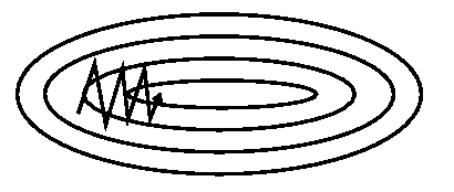
Momentum

Unfortunately, even with these normalization tricks, ill-conditioned curvature is a fact of life. We need algorithms that are able to deal with it.
Momentum:

$$\begin{eqnarray} \mathbf{v}_t &=& \gamma\mathbf{v}_{t-1} + \alpha\nabla_{\mathbf{\theta}}J(\mathbf{\theta}) \nonumber \\ \mathbf{\theta}_t &=& \mathbf{\theta}_{t-1} - \mathbf{v}_t \nonumber \end{eqnarray}$$

Nesterov Accelerated Gradient:

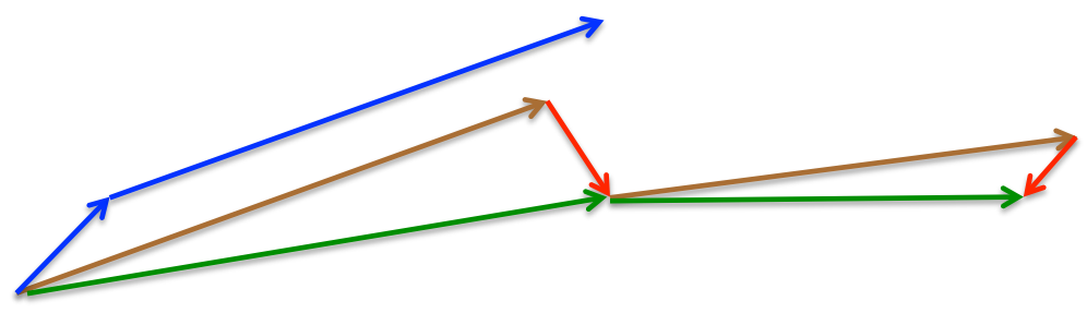
$$\begin{eqnarray} \mathbf{v}_t &=& \gamma\mathbf{v}_{t-1} + \alpha\nabla_{\mathbf{\theta}}J(\mathbf{\theta-\gamma\mathbf{v}_{t-1}}) \nonumber \\ \mathbf{\theta}_t &=& \mathbf{\theta}_{t-1} - \mathbf{v}_t \nonumber \end{eqnarray}$$

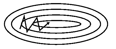
Why Momentum

In the high curvature directions, the gradients cancel each other out, so momentum dampens the oscillations.
In the low curvature directions, the gradients point in the same direction, allowing the parameters to pick up speed.
If the gradient is constant (i.e. the cost surface is a plane), the parameters will reach a terminal velocity of

$$ -\frac{\alpha}{1-\gamma}\cdot \frac{\partial \mathcal{L}}{\partial \mathbf{\theta}} $$

This suggests if you increase $\gamma$, you should lower $\alpha$ to compensate.
Momentum sometimes helps a lot, and almost never hurts.

Adam

Adapt learning rate by using moments of gradients
First and Second Order Moments:

$$ \begin{eqnarray} \mathbf{m}_t &=& \beta_1 \mathbf{m}_{t-1} + (1-\beta_1)\mathbf{g}_t \\ \mathbf{v}_t &=& \beta_1 \mathbf{v}_{t-1} + (1-\beta_1)\mathbf{g}^2_t \end{eqnarray} $$

Bias Correction:

$$ \begin{eqnarray} \mathbf{\hat{m}}_t = \frac{\mathbf{m}_t}{1-\beta_1} \nonumber \\ \mathbf{\hat{v}}_t = \frac{\mathbf{v}_t}{1-\beta_1} \nonumber \end{eqnarray} $$

Adam Update:

$$ \begin{equation} \mathbf{\theta}_t = \mathbf{\theta}_{t-1} - \frac{\alpha}{\sqrt{\mathbf{\hat{v}}_t+\epsilon}}\mathbf{\hat{m}}_t \end{equation} $$

$L_2$ Regularization vs Weight Decay

$L_2$ regularization and weight decay are equivalent for SGD and SGD+Momentum.
But they are not the same for adaptive methods (AdaGrad, RMSprop, Adam etc.)
AdamW decouples weight decay.

It should be your default optimizer

In Practice...

Adam/AdamW is a good default choice.
In many cases SGD+Momentum can outperform Adam but may require more tuning.
If you can afford to do full batch updates, then try out L-BFGS.