Autoregressive Models

CSE 891: Deep Learning

Vishnu Boddeti

Wednesday November 11, 2020

A Probabilistic Viewpoint

Goal: modeling $p_{data}$

Fully Observed Models

Transformation Models (likelihood free)

Latent Variable Models (observation noise)

Undirected Latent Variable Models (hidden factors)

Bayes Nets and Neural Nets

Key idea: place a Bayes net structure (a directed acyclic graph) over the variables in the data, and model the conditional distributions with neural networks.
Reduces the problem to designing conditional likelihood-based models for single variables.

We know how to do this: the neural net takes variables being conditioned on as input, and outputs the distribution for the variable being predicted.

Autoregressive Models

First, given a Bayes net structure, setting the conditional distributions to neural networks will yield a tractable log likelihood and gradient. Great for maximum likelihood training! \begin{equation} \log p_{\theta}(\mathbf{x}) = \sum_{i=1}^d \log p_{\theta}(x_i|parents(x_i)) \end{equation}
But is it expressive enough? Yes, assuming a fully expressive Bayes net structure: any joint distribution can be written as a product of conditionals \begin{equation} \log p(\mathbf{x}) = \sum_{i=1}^d \log p(x_i|x_{1:i-1}) \end{equation}
This is called an autoregressive model. So, an expressive Bayes net structure with neural network conditional distributions yields an expressive model for p(x) with tractable maximum likelihood training.

Toy Autoregressive Model

Two variables: $x_1$, $x_2$
Model: $p(x_1, x_2) = p(x_1) p(x_2|x_1)$
$p(x_1)$ is a histogram
$p(x_2|x_1)$ is a multilayer perceptron

Input is $x_1$
Output is a distribution over $x_2$ (logits, followed by softmax)

Fully Observed Models

Direct data modeling
No latent variables
Example: Recurrent Neural Networks
All conditional probabilities described by deep networks

$$\begin{equation} \begin{aligned} x_1 &\sim Cat(x_1|\pi) \\ x_2 &\sim Cat(x_2|\pi(x_1)) \\ & \dots \\ x_n &\sim Cat(x_n|\pi(\mathbf{x}_{< n})) \\ p(\mathbf{x}) &= \prod_{i} p(x_i|f(\mathbf{x}_{< i};\mathbf{\theta})) \\ \end{aligned} \end{equation}$$

One Function Approximator Per Conditional

Does this extend to high dimensions?

Somewhat. For d-dimensional data, $\mathcal{O}(d)$ parameters

Much better than $\mathcal{O}(\exp(d))$ in tabular case
What about text generation where $d$ can be arbitrarily large?

Limited generalization

No information sharing among different conditionals

Solution: share parameters among conditional distributions. Two approaches:

Recurrent neural networks
Masking

Recurrent Neural Networks

RNN as Autoregressive Models

\begin{equation} \log p(\mathbf{x}) = \sum_{i=1}^d \log p(x_i|x_{1:i-1}) \end{equation}

MNIST

Handwritten digits
$28\times28$
60,000 train
10,000 test

Original: grayscale
"Binarized MNIST": 0/1 (black/white)

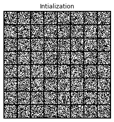
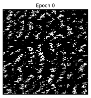
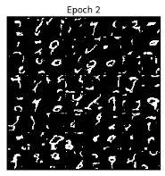
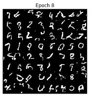
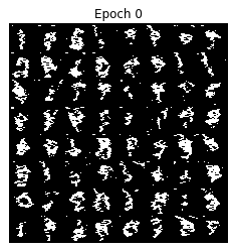
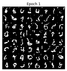
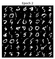
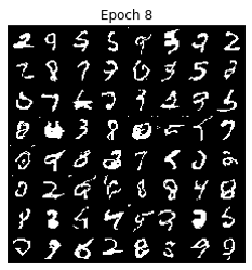
RNN on MNIST

RNN with Pixel Location Appended on MNIST

Append $(x,y)$ coordinates of pixel in the image as input to RNN

Masking

Masking Based Autoregressive Models

Second major branch of neural AR models

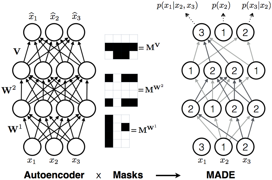
Key property: parallelized computation of all conditionals
Masked MLP (MADE)
Masked convolutions & self-attention

Also share parameters across time

Masked Autoencoder for Distribution Estimation (MADE)

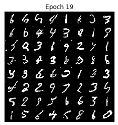
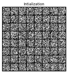
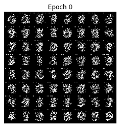
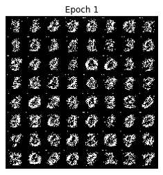
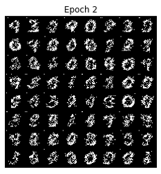
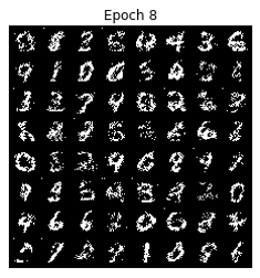
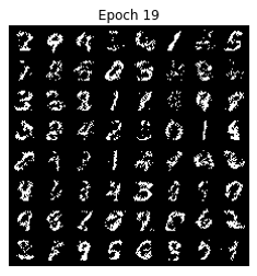
MADE on MNIST

MADE Results

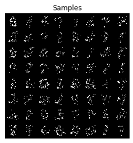
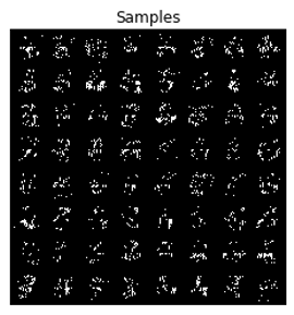
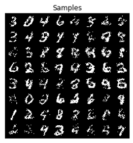
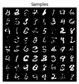
MADE -- Different Orderings

Random Permutation

Even-Odd Indices

Row (raster scan)

Columns

Top to Middle + Bottom to Middle

Masked Temporal (1D) Convolution

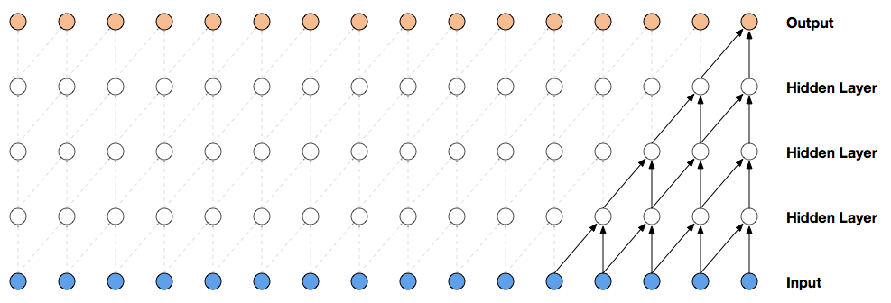
Easy to implement, masking part of the conv kernel
Constant parameter count for variable-length distribution!
Efficient to compute, convolution has hyper-optimized implementations on all hardware
However

Limited receptive field, linear in number of layers

WaveNet

Improved receptive field: dilated convolution, with exponential dilation
Better expressivity: Gated Residual blocks, Skip connections

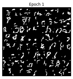
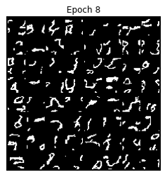
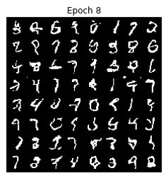
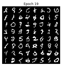
WaveNet on MNIST

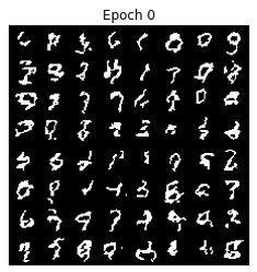
WaveNet with Pixel Location Appended on MNIST

Append $(x,y)$ coordinates of pixel in the image as input to RNN

Masked Spatial (2D) Convolution - PixelCNN

Images can be flatten into 1D vectors, but they are fundamentally 2D
We can use a masked variant of ConvNet to exploit this knowledge
First, we impose an autoregressive ordering on 2D images:

This is called raster scan ordering. (Different orderings are possible, more on this later)

PixelCNN

Design question: how to design a masking method to obey that ordering?
One possibility: PixelCNN (2016)

PixelCNN

PixelCNN-style masking has one problem: blind spot in receptive field

Gated PixelCNN

Gated PixelCNN (2016) introduced a fix by combining two streams of convolutions

Gated PixelCNN

Improved ConvNet architecture: Gated ResNet Block

\[\mathbf{y} = \mbox{tanh}(\mathbf{W}_{k,f}\ast\mathbf{x})\odot\sigma(\mathbf{W}_{k,g}\ast\mathbf{x})\]

Gated PixelCNN

Better receptive field + more expressive architecture = better performance

PixelCNN++

Moving away from softmax: we know nearby pixel values are likely to co-occur!

\begin{eqnarray} \nu &\sim& \sum_{i=1}^K \pi_i logistic(\mu_i, s_i) \\ P(x|\pi,\mu,s) &=& \sum_{i=1}^K \pi_i\left[\sigma\left(\frac{x+0.5-\mu_i}{s_i}\right)-\sigma\left(\frac{x-0.5-\mu_i}{s_i}\right)\right] \end{eqnarray}

Recap: Logistic distribution

Training Mixture of Logistics

PixelCNN++

Capture long dependencies efficiently by downsampling

PixelCNN++

Masked Attention

A recurring problem for convolution: limited receptive field $\rightarrow$ hard to capture long-range dependencies
Self-Attention: an alternative that has

unlimited receptive field!!
also $\mathcal{O}(1)$ parameter scaling w.r.t. data dimension
parallelized computation (versus RNN)

Masked Attention

Much more flexible than masked convolution. We can design any autoregressive ordering we want
An example:

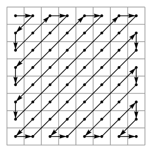
Zigzag Ordering

How to implement with masked conv?
Trivial to do with masked attention!

Masked Attention + Convolution

Gated PixelCNN

PixelCNN++

PixelSNAIL

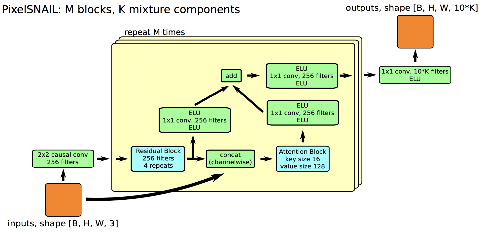
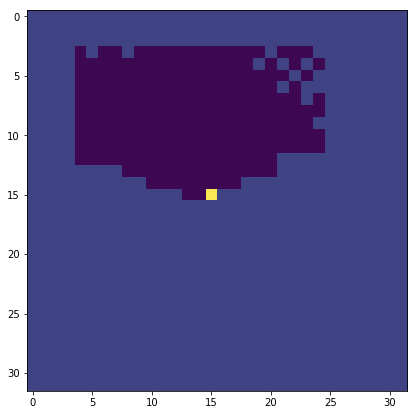
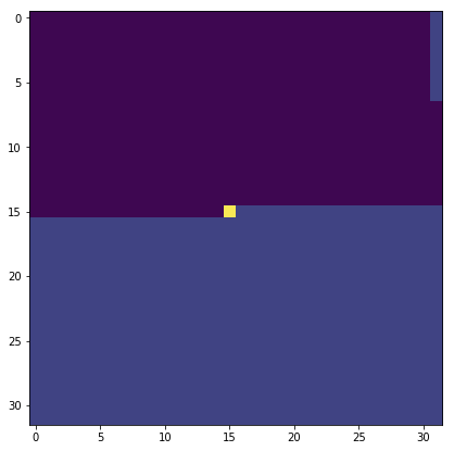
Masked Attention + Convolution

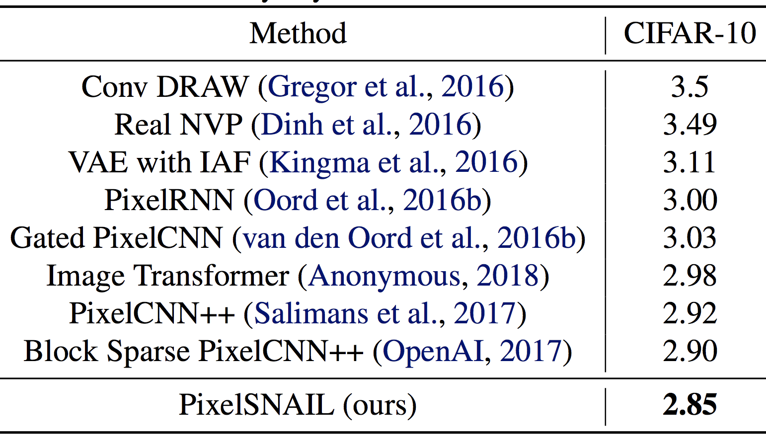
Class Conditional PixelCNN

How to condition?

Input: One-hot encoding of the labels
Then: multiplying by different learned weight matrices in each convolutional layer, and added as a bias channel-wise and broadcasted spatially

Hierarchical Autoregressive Models with Auxiliary Decoders

Image Super-Resolution with PixelCNN

A PixelCNN is conditioned on $7 \times 7$ subsampled MNIST images to generated the corresponding $28 \times 28$ image

Pixel Recursive Super Resolution

Neural Autoregressive Models: The Good

Can directly encode how observed points are related.
Any data type can be used
For directed graphical models: Parameter learning simple
Log-likelihood is directly computable, no approximation needed.
Easy to scale-up to large models, many optimization tools available.
Best in class modelling performance:

expressivity - autoregressive factorization is general
generalization - meaningful parameter sharing has good inductive bias

State of the art models on multiple datasets, modalities

Neural Autoregressive Models: The Bad

Order sensitive.
For undirected models, parameter learning difficult: Need to compute normalizing constants.
Generation can be slow: iterate through elements sequentially, or using a Markov chain.

Sampling each pixel = 1 forward pass!
11 minutes to generate 16 32-by-32 images on a Tesla K40 GPU

Solutions

Faster implementation
Speedup by breaking autoregressive pattern: create groups of pixels

$\mathcal{O}(d) \rightarrow \mathcal{O}(\log(d))$ by parallelizing within groups.