Uninformed Search
CSE 440: Introduction to Artificial Intelligence
Content Credits: CMU AI, http://ai.berkeley.edu
Today
- Uninformed Search
- Search Trees
- Search Algorithm Properties
- Depth First Search
- Breadth First Search
- Uniform Cost Search

- Reading
- Today's Lecture: RN Chapter 3.1-3.4
- Next Lecture: RN Chapter 3.5-3.7, 4.1-4.2
State Space Graphs and Search Trees
State Space Graphs
- State Space Graph: A mathematical representation of a search problem
- Nodes are (abstracted) world configurations
- Arcs represent successors (action results)
- The goal test is a set of goal nodes (maybe only one)
- In a state space graph, each state occurs only once
- We can rarely build this full graph in memory (too big), but it is a useful idea

Search Trees


- A search tree :
- A "what if" tree of plans and their outcomes
- The start state is the root node
- Child nodes correspond to successors
- Nodes show states, but correspond to plans/actions that achieve those states
- Building the whole tree is impossible for most problems
State Space vs Search Trees


- Each NODE in search tree is an entire PATH in state space graph.
- Construct both on demand – and construct as little as possible.
Tree Search
Search Example: Traveling in Romania
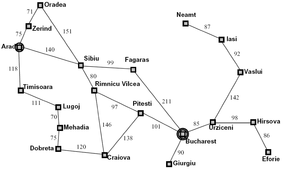
Search Tree: Traveling in Romania
- Search:
- Expand out potential plans (tree nodes)
- Maintain a fringe of partial plans under consideration
- Try to expand as few tree nodes as possible
Tree Search Algorithm

- Important Ideas:
- Fringe
- Expansion
- Exploration Strategy
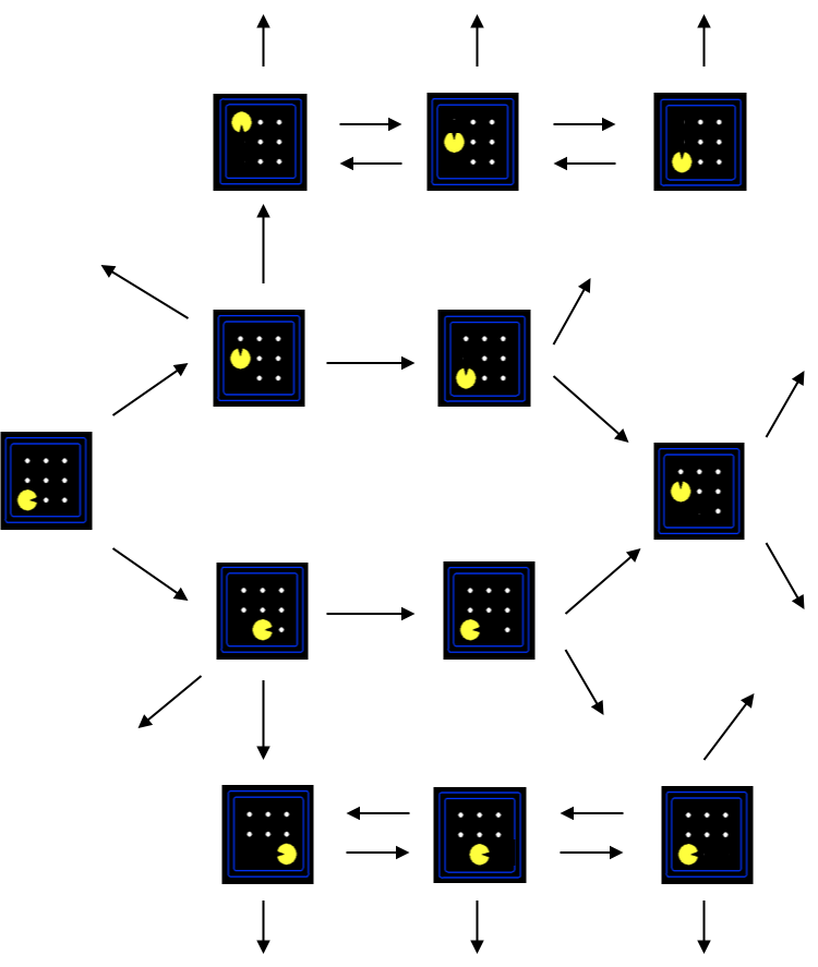
Tree Search Example


Search Algorithm Properties
Search Algorithm Properties
- Complete: Guaranteed to find a solution if one exists?
- Optimal: Guaranteed to find the least cost path?
- Time Complexity?
- Space Complexity
- Cartoon of search tree:
- $b$ is the branching factor
- $m$ is the maximum depth
- solutions at various depths
- Number of nodes in a tree?
- $1+b+b^2+\cdots+b^m=\mathcal{O}(b^m)$


Depth-First Search
Depth First Search


- Strategy: expand the deepest node first
- Implementation: fringe is a FILO or LIFO stack
Depth-First Search (DFS) Properties
- What nodes DFS expand?
- Some left prefix of the tree.
- Could process the whole tree!
- If $m$ is finite, takes time $\mathcal{O}(b^m)$


- Is it complete?
- $m$ could be infinite, so only if we prevent cycles (more later)
- How much space does the fringe take?
- Only has siblings on path to root, so $\mathcal{O}(bm)$.
- Is it optimal?
- No, it finds the "leftmost" solution, regardless of depth or cost.
Breadth-First Search
Breadth First Search


- Strategy: expand the shallowest node first
- Implementation: fringe is a FIFO queue
Breadth-First Search (BFS) Properties
- What nodes BFS expand?
- Processes all nodes above shallowest solution
- Let depth of shallowest solution be $s$
- Search takes time $\mathcal{O}(b^s)$
- How much space does the fringe take?
- Roughly the last tier, so $\mathcal{O}(b^s)$.
- Is it complete?
- $s$ must be finite if a solution exists, so yes!
- Is it optimal?
- Only if costs are all 1 (more on costs later)


Iterative Deepening
- Idea: get the space advantage of DFS with the time / shallow-solution advantage of BFS.
- Run a DFS with depth limit 1. If no solution $\dots$
- Run a DFS with depth limit 2. If no solution $\dots$
- Run a DFS with depth limit 3. If no solution $\dots$
- Is this not wastefully redundant?
- Generally most work happens in the deepest level searched, so it is not so bad.
Cost Sensitive Search

Uniform Cost Search
Uniform Cost Search (UCS)


- Strategy: expand a cheapest node first
- Implementation: fringe is a priority queue (priority: cumulative cost)
UCS Properties
- What nodes UCS expand?
- Processes all nodes with cost less than cheapest solution!
- If that solution costs $C^*$ and arcs cost at least $\epsilon$ , then the "effective depth" is roughly $\left(\frac{c^*}{\epsilon}\right)$
- Takes time $\mathcal{O}\left(b^{\frac{C^*}{\epsilon}}\right)$ (exponential in effective depth)
- How much space does the fringe take?
- Has roughly the last tier, so $\mathcal{O}\left(b^{\frac{C^*}{\epsilon}}\right)$


- Is it complete?
- Assuming best solution has a finite cost and minimum arc cost is positive, yes!
Uniform Cost Issues
- Remember: UCS explores increasing cost contours
- The good: UCS is complete and optimal!
- The bad:
- Explores options in every "direction"
- No information about goal location
- Will be addressed soon.


UCS Demo
The One Queue
- All these search algorithms are the same except for fringe strategies
- Conceptually, all fringes are priority queues (i.e. collections of nodes with attached priorities)
- Practically, for DFS and BFS, you can avoid the $log(n)$ overhead from an actual priority queue, by using stacks and queues
- Can even code one implementation that takes a variable queuing object
Search and Models
- Search operates over models of the world
- The agent does not actually try all the plans out in the real world.
- Planning is all "in simulation"
- Your search is only as good as your models
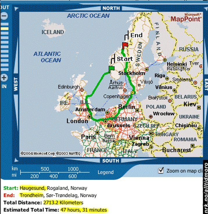
Search Gone Wrong?

Q & A