Bayesian Networks: Inference
CSE 440: Introduction to Artificial Intelligence
Vishnu Boddeti
Content Credits: CMU AI, http://ai.berkeley.edu
Today
- Bayes Net Inference
- Factors
- Variable Elimination
Bayes Net Representation
- A directed, acyclic graph, one node per random variable
- A conditional probability table (CPT) for each node
- A collection of distributions over $X$, one for each combination of parents values
\[P(X|a_1,\dots,a_n)\]
- Bayes nets implicitly encode joint distributions
- As a product of local conditional distributions
- To see what probability a BN gives to a full assignment, multiply all the relevant conditionals together:
\[P(x_1,\dots,x_n)=\prod_{i=1}^nP(x_i|parents(x_i))\]
What is Inference?
- Inference: calculating some useful quantity from a joint probability distribution
- Example:
- Posterior Probability:
\[P(Q|E_1=e_1,\dots,E_k=e_k)\]
- Most likely explanation:
\[\underset{q}{\operatorname{arg max}} P(Q|E_1=e_1,\dots,E_k=e_k)\]
Inference by Enumeration
- Problem Setup:
- General Case:
- Evidence variables: $E_1,\dots,E_k=e_1,\dots,e_k$
- Query variables: $Q$
- Hidden variables: $H_1,\dots,H_r$
- We want: $P(Q|e_1\dots,e_k)$
- Solution:
- Step 1: Select the entries consistent with the evidence
- Step 2: Sum out $H$ to get joint of Query and evidence
\[P(Q,e_1\dots,e_k)=\sum_{h_1,\dots,h_r}P(Q,h_1,\dots,h_r,e_1,\dots,e_k)\]
- Step 3: Normalize
\[Z = \sum_{q} P(Q,e_1,\dots,e_r)\]
\[P(Q|e_1\dots,e_r) = \frac{1}{Z}P(Q,e_1,\dots,e_r)\]
Inference by Enumeration in Bayes Net
- Given unlimited time, inference in BNs is easy
- Reminder of inference by enumeration by example:
\begin{equation}
\begin{aligned}
P(B|+j,+m) &\propto P(B,+j,+m) \nonumber \\
&= \sum_{e,a} P(B,e,a,+j,+m) \nonumber \\
&= \sum_{e,a} P(B)P(e)P(a|B,e)P(+j|a)P(+m|a) \nonumber \\
\end{aligned}
\end{equation}
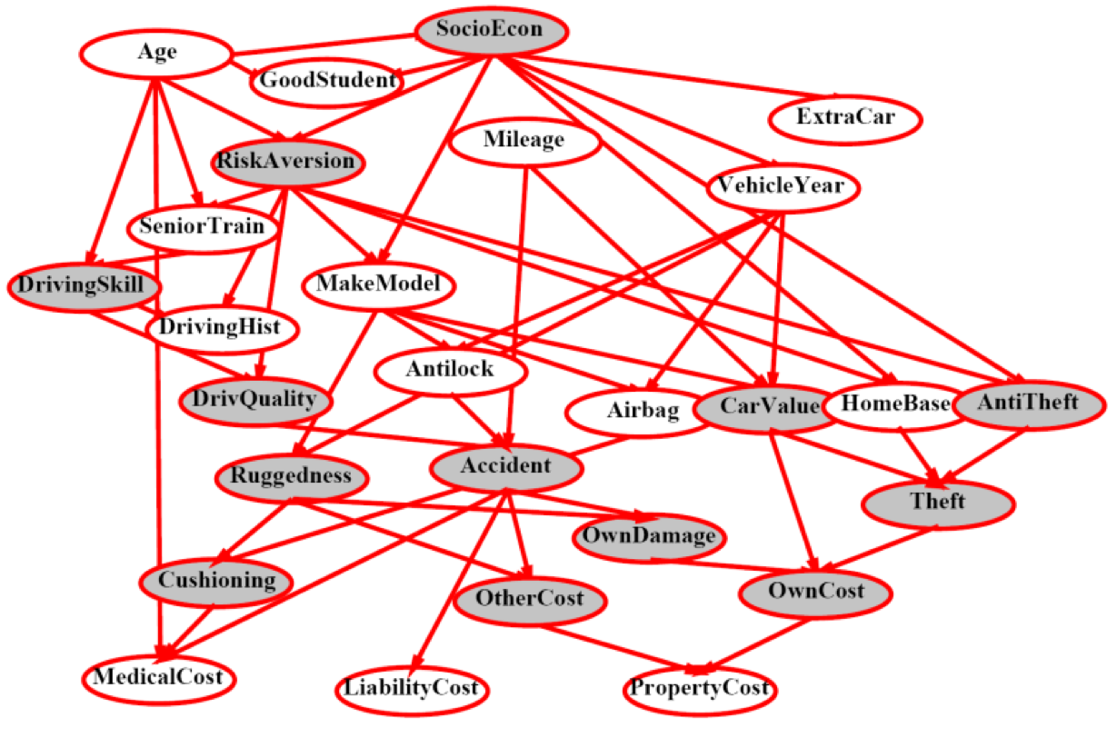
Inference by Enumeration?

Inference by Enumeration vs Variable Elimination
- Why is inference by enumeration so slow?
- You join up the whole joint distribution before you sum out the hidden variables
- Idea: interleave joining and marginalizing
- Called "Variable Elimination"
- Still NP-hard, but usually much faster than inference by enumeration
- First we will need some new notation: factors
Factors I
- Joint distribution: P(X,Y)
- Entries $P(x,y)$ for all $x$, $y$
- Sums to 1
- Selected joint: $P(x,Y)$
- A slice of the joint distribution
- Entries $P(x,y)$ for fixed $x$, all $y$
- Sums to $P(x)$
- Number of capitals = dimensionality of the table
$P(T,W)$
| $T$ |
$W$ |
$P$ |
| hot |
sun |
0.4 |
| hot |
rain |
0.1 |
| cold |
sun |
0.2 |
| cold |
rain |
0.3 |
$P(cold,W)$
| $T$ |
$W$ |
$P$ |
| cold |
sun |
0.2 |
| cold |
rain |
0.3 |
Factors II
- Single conditional: $P(Y|x)$
- Entries $P(y|x)$ for fixed $x$, all $y$
- Sums to 1
- Family of conditionals: $P(Y|X)$
- Multiple conditionals
- Entries $P(y|x)$ for all $x$, $y$
- Sums to $|X|$
$P(W|cold)$
| $T$ |
$W$ |
$P$ |
| cold |
sun |
0.4 |
| cold |
rain |
0.6 |
$P(W|T)$
| $T$ |
$W$ |
$P$ |
| hot |
sun |
0.8 |
| hot |
rain |
0.2 |
| cold |
sun |
0.4 |
| cold |
rain |
0.6 |
Factors III
- Specified family: $P(y|X)$
- Entries $P(y|x)$ for fixed $y$, but for all $x$
- Sums to $\dots$ who knows
$P(rain|T)$
| $T$ |
$W$ |
$P$ |
| hot |
rain |
0.2 |
| cold |
rain |
0.6 |
Factors Summary
- In general, when we write $P(Y_1,\dots,Y_N|X_1,\dots,X_M)$
- It is a "factor," a multi-dimensional array
- Its values are $P(y_1,\dots,y_N|x_1,\dots,x_M)$
- Any assigned (=lower-case) $X$ or $Y$ is a dimension missing (selected) from the array
Example: Traffic Domain
- Random Variables
- R: raining
- T: traffic
- L: late for class
\begin{equation}
\begin{aligned}
P(L) &= ? \nonumber \\
&= \sum_{r,t} P(r,t,L) \nonumber \\
&= \sum_{r,t} P(r)P(t|r)P(L|t) \nonumber
\end{aligned}
\end{equation}
Inference by Enumeration: Procedural Outline
- Track objects called factors
- Initial factors are local CPTs (one per node)
- Any known values are selected
- E.g. if we know $L=+l$, the initial factors are
- Procedure: Join all factors, eliminate all hidden variables, normalize
Operation 1: Join Factors
- First basic operation: joining factors
- Combining factors:
- Just like a database join
- Get all factors over the joining variable
- Build a new factor over the union of the variables involved
- Example: Join on R
- Computation for each entry: pointwise products $\forall r,t \mbox{ : } P(r,t)=P(r)P(t|r)$
Operation 2: Eliminate
- Second basic operation: marginalization
- Take a factor and sum out a variable
- Shrinks a factor to a smaller one
- A projection operation
- Example:
Thus Far
Multiple Join, Multiple Eliminate (= Inference by Enumeration)
Variable Elimination
(Marginalizing Early)
Traffic Domain

- Inference by Enumeration
\begin{equation}
=\sum_{t}\sum_{r}P(L|t)P(r)P(t|r) \nonumber
\end{equation}
- join $r$
- join $t$
- eliminate $r$
- eliminate $t$
- Variable Elimination
\begin{equation}
=\sum_{t}P(L|t)\sum_{r}P(r)P(t|r) \nonumber
\end{equation}
- join $r$
- eliminate $r$
- join $t$
- eliminate $t$
Evidence I
- If evidence, start with factors that select that evidence
- No evidence uses these initial factors:

- Computing $P(L|+r)$, the initial factors become:
- We eliminate all vars other than query + evidence
Evidence II
- Result will be a selected joint of query and evidence
- E.g. for $P(L|+r)$, we would end up with:
- To get our answer, just normalize this
- That is it
General Variable Elimination
- Query: $P(Q|E_1=e_1,\dots,E_k=e_k)$
- Start with initial factors:
- Local CPTs (but instantiated by evidence)
- While there are still hidden variables (not Q or evidence):
- Pick a hidden variable $H$
- Join all factors mentioning $H$
- Eliminate (sum out) $H$
- Join all remaining factors and normalize
Example
- Estimate $P(B|+j,+m)$
- We have access to:
- $P(B)$, $P(E)$, $P(A|B,E)$, $P(+j|A)$, $P(+m|A)$
Example Continued...
- Estimate $P(B|+j,+m)$
- We have access to:
- $P(B)$, $P(E)$, $P(+j,+m|B,E)$
Variable Elimination Ordering

- For the query $P(X_n|y_1,\dots,y_n)$ work through the following two different orderings as done in previous slide:
- $Z, X_1, \dots, X_{n-1}$
- $X_1, \dots, X_{n-1}, Z$.
- What is the size of the maximum factor generated for each of the orderings?
- Answer: $2^{n+1}$ vs $2^2$ (for binary)
- In general: the ordering can greatly affect efficiency.
VE: Computational and Space Complexity
- The computational and space complexity of variable elimination is determined by the largest factor
- The elimination ordering can greatly affect the size of the largest factor.
- E.g., example on previous slide $2^n$ vs. $2$
- Does there always exist an ordering that only results in small factors?


