Feed Forward Networks: Learning
CSE 891: Deep Learning
Monday September 13, 2021
Today
- Risk Minimization
- Loss Functions
- Regularization
Recap
Recap: Simple Neural Network
- Neuron pre-activation (or input activation)
- $a(\mathbf{x}) = b + \sum_i w_ix_i = b + \mathbf{w}^T\mathbf{x}$
- Neuron (output) activation $h(\mathbf{x}) = g(a(\mathbf{x})) = g\left(b+\sum_iw_ix_i\right)$
- $\mathbf{w}$ are the connection weights
- $b$ is the neuron bias
- $g(\cdot)$ is called activation function

Recap: Multilayer Neural Network
- Could have $L$ hidden layers:
- layer pre-activation for $k>0$ ($\mathbf{h}^{(0)}(\mathbf{x})=\mathbf{x}$) $\mathbf{a}^{(k)}(\mathbf{x}) = \mathbf{b}^{(k)} + \mathbf{W}^{(k)}\mathbf{h}^{(k-1)}(\mathbf{x})$
- hidden layer activation ($k$ from 1 to $L$): $\mathbf{h}^{(k)}(\mathbf{x}) = \mathbf{g}(\mathbf{a}^{(k)}(\mathbf{x}))$
- output layer activation ($k=L+1$): $\mathbf{h}^{(L+1)}(\mathbf{x}) = \mathbf{o}(\mathbf{a}^{(L+1)}(\mathbf{x})) = f(\mathbf{x})$

Risk Minimization
Empirical Risk Minimization
- Framework to design learning algorithms $$\underset{\theta}{\operatorname{arg min}} \mathbb{E}_{P(x,y)}\left[l\left(f(\mathbf{x}^t;\mathbf{\theta}),\mathbf{y}^t\right)\right] + \lambda\Omega(\mathbf{\theta})$$ $$\underset{\theta}{\operatorname{arg min}} \frac{1}{T} \sum_t l\left(f(\mathbf{x}^t;\mathbf{\theta}),\mathbf{y}^t\right) + \lambda\Omega(\mathbf{\theta})$$
- Learning is cast as an optimization problem
- Loss Function: $l(f(\mathbf{x}^t;\mathbf{\theta}),\mathbf{y}^t)$
- $\Omega(\mathbf{\theta})$ is a regularizer
Log-Likelihood
- NN estimates $f(\mathbf{x})_c=p(y=c|\mathbf{x})$
- we could maximize the probabilities of $y_t$ given $\mathbf{x}_t$ in the training set
- To frame as minimization, we minimize the negative log-likelihood $$l(f(\mathbf{x}),y) = -\log \sum_c 1_{y=c}f(\mathbf{x})_c = -\log f(\mathbf{x})_y$$
- we take the log to simplify numerical stability and math simplicity
- sometimes referred to as cross-entropy
Loss Functions
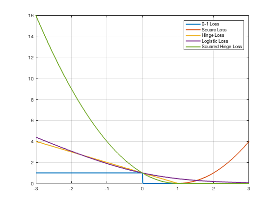
Loss Functions: Classification
- $l(\hat{y},y) = \sum_i \mathcal{I}(\hat{y}_i \neq y_i)$
- Surrogate Loss Functions:
- Squared Loss: $\left(y-f(\mathbf{x})\right)^2$
- Logistic Loss: $\log\left(1+e^{-yf(\mathbf{x})}\right)$
- Hinge Loss: $\left(1-yf(\mathbf{x})\right)_+$
- Squared Hinge Loss: $\left(1-yf(\mathbf{x})\right)_+^2$
- Cross-Entropy Loss: $-\sum_{i} y_i\log f(\mathbf{x})_i$
Loss Functions: Regression
- Euclidean Loss: $\|\mathbf{y}-f(\mathbf{x})\|_2^2$
- Manhattan Loss: $\|\mathbf{y}-f(\mathbf{x})\|_1$
- Huber Loss: $$ \begin{cases} \frac{1}{2}\|\mathbf{y}-f(\mathbf{x})\|_2^2 & \quad \text{for } \|\mathbf{y}-f(\mathbf{x})\| < \delta\\ \delta\|\mathbf{y}-f(\mathbf{x})\|_1 -\frac{1}{2}\delta^2 & \quad \text{otherwise}\\ \end{cases} $$
- KL Divergence: $\sum_i p_ilog\left(\frac{p_i}{q_i}\right)$

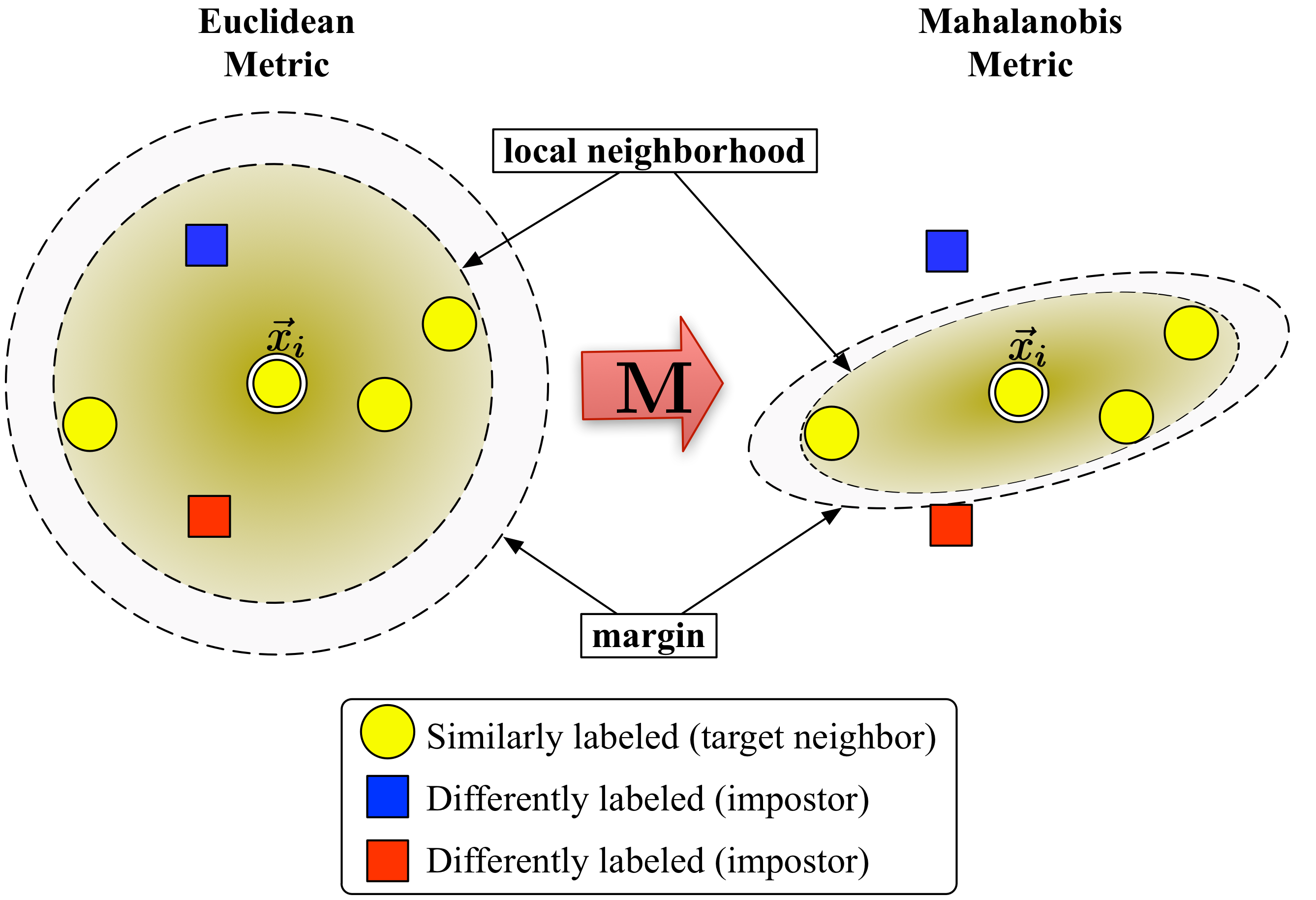
Loss Functions: Embeddings
- Cosine Distance: $\frac{\mathbf{x}^T\mathbf{y}}{\|x\|\|y\|}$
- Triplet Loss: $\left(1+d(\mathbf{x}_i,\mathbf{x}_j)-d(\mathbf{x}_i,\mathbf{x}_k)\right)_{+}$
- Mahalanobis Distance: $(\mathbf{x}-\mathbf{y})^T\mathbf{M}(\mathbf{x}-\mathbf{y})$
Cross-Entropy Loss Example
| Unnormalized Log-Prob | Unnormalized Prob. | Prob. | Correct Prob |
|---|---|---|---|
| 3.2 | 24.5 | 0.13 | 1.00 |
| 5.1 | 164.0 | 0.87 | 0.00 |
| -1.7 | 0.18 | 0.00 | 0.00 |
Regularization
Regularization
- What is regularization?
- the process of constraining the parameter space
- alternatively, penalize certain values of $\mathbf{\theta}$
- Why do we need regularization?
- In Machine Learning regularization $\Leftrightarrow$ generalization
- In Deep Learning regularization $\neq$ generalization
$L_2$ Regularization
$$\Omega(\mathbf{\theta}) = \sum_k\sum_i\sum_j(W_{ij}^k)^2 = \sum_k\|\mathbf{W}^k\|_F^2$$- Gradient: $\nabla_{\mathbf{W}^k}\Omega(\mathbf{\theta}) = 2\mathbf{W}^k$
- Only applied on weights, not on biases (weight decay)
- Can be interpreted as having a Gaussian prior over the weights
$L_1$ Regularization
$$\Omega(\mathbf{\theta}) = \sum_k\sum_i\sum_j|W_{ij}^k|$$- Gradient: $\nabla_{\mathbf{W}^k}\Omega(\mathbf{\theta}) = sign(\mathbf{W}^k)$ $$sign(W^k)_{i,j} = \begin{cases} 1 & \quad \text{for } W^k_{ij} > 0\\ -1 & \quad \text{for } W^k_{ij} < 0 \end{cases}$$
- Only applied on weights, but not to biases
- Unlike $L_2$, $L_1$ will push certain weights to be exactly zero
- Can be interpreted as having a Laplacian prior over the weights
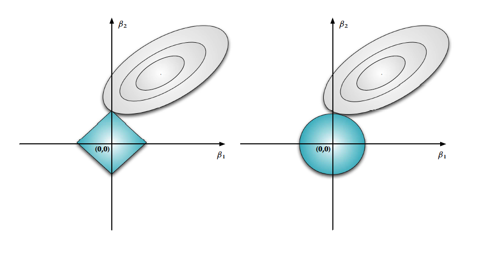
Regularization Geometry
Equivalent Optimization Problems: $$ \begin{equation} \textbf{P1: } \underset{\mathbf{W}}{\operatorname{arg max}} \||\mathbf{y}-\mathbf{W}\mathbf{x}\||_2^2 + \lambda\||\mathbf{W}\||_2^2 \end{equation} $$ $$ \begin{eqnarray} \textbf{P2: } \underset{\mathbf{W}}{\operatorname{arg max}} && \||\mathbf{W}\||_2^2 \nonumber \\ s.t. && \||\mathbf{y}-\mathbf{W}\mathbf{x}\||_2^2 \leq \alpha \nonumber \end{eqnarray} $$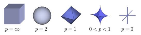
Looking Through the Bayesian Lens
- Bayes Rule: $$ \begin{eqnarray} p(\mathbf{\theta}|\mathbf{x},\mathbf{y}) &=& \frac{p(\mathbf{y}|\mathbf{x},\mathbf{\theta})p(\mathbf{\theta})}{p(\mathbf{y}|\mathbf{x})} \\ &=& \frac{p(\mathbf{y}|\mathbf{x},\mathbf{\theta})p(\mathbf{\theta})}{\int_{\mathbf{\theta}}p(\mathbf{y}|\mathbf{x},\mathbf{\theta})p(\mathbf{\theta})} \end{eqnarray} $$
- Likelihood: $$ p(\mathbf{y}|\mathbf{x},\mathbf{\theta}) = \frac{1}{Z}e^{-E(\mathbf{\theta},\mathbf{x},\mathbf{y})} $$
- Prior: $$p(\mathbf{\theta}) = \frac{1}{Z}e^{-E(\mathbf{\theta})}$$
Maximum-Aposteriori-Learning (MAP)
$$ \begin{eqnarray} \hat{\mathbf{\theta}} &=& \underset{\theta}{\operatorname{arg max}} \prod_i p(\mathbf{\theta}|\mathbf{x}_i,\mathbf{y}_i) \nonumber \\ \end{eqnarray} $$ $$ \begin{eqnarray} &=& \underset{\theta}{\operatorname{arg max}} p(\mathbf{\theta})\frac{\prod_i p(\mathbf{y}_i|\mathbf{x}_i,\mathbf{\theta})}{\prod_i p(\mathbf{y}_i|\mathbf{x}_i)} \nonumber \\ \end{eqnarray} $$ $$ \begin{eqnarray} &=& \underset{\theta}{\operatorname{arg max}} p(\mathbf{\theta})\prod_i p(\mathbf{y}_i|\mathbf{x}_i,\mathbf{\theta}) \nonumber \\ \end{eqnarray} $$ $$ \begin{eqnarray} &=& \underset{\theta}{\operatorname{arg min}} \left(E(\mathbf{\theta},\mathbf{x},\mathbf{y}) + E(\mathbf{\theta})\right) \nonumber \end{eqnarray} $$- Example:
Q & A