Automatic Differentiation

CSE 891: Deep Learning

Vishnu Boddeti

Monday September 20, 2021

Implementing Backpropagation

Implementing backpropagation by hand is like doing assembly programming.

You don't have to do it most of the times.
You need it sometimes, when desired functionality is absent.
You do need it sometimes, if you want to eke out all the efficiencies out of the hardware.

Can we automate the process of computing gradients of arbitrary functions?
Autodiff: An automatic differentiation library.

Terminology

Automatic Differentiation (AutoDiff): A general purpose solution for taking a program that computes a scalar value and automatically constructing a procedure for the computing the derivative of that value.

Forward Mode Autodiff
Reverse Mode Autodiff

Backpropagation: A special case of autodiff applied to neural networks. The words "backpropagation" and "autodiff" are used interchangeably in machine learning.
AutoGrad: It is the name of a particular autodiff package.

Finite Differences

We often use finite differences to check our gradient calculations.
One-sided version: $\begin{equation}\frac{\partial}{\partial x_i}f(x_1,\dots,x_N)\approx\frac{f(x_1,\dots,x_i+h,\dots,x_N)-f(x_1,\dots,x_i,\dots,x_N)}{h}\end{equation}$
Two-sided version: $\begin{equation}\frac{\partial}{\partial x_i}f(x_1,\dots,x_N)\approx\frac{f(x_1,\dots,x_i+h,\dots,x_N)-f(x_1,\dots,x_i-h,\dots,x_N)}{2h}\end{equation}$

What Autodiff is not...

Finite Difference Approximation

Computationally expensive, needs many forward passes.
Can induce large numerical errors.
Normally, we only use it for testing.

Symbolic Differentiation

Can result in complex and redundant expressions.
There may not be a convenient formula for the derivative.

What Autodiff is...

An efficient (linear in the cost of computing the scalar value) and numerically stable way of computing gradients.
A procedure for computing the derivatives, as opposed to obtaining a formula.

Recap: Derivative Example

Forward Pass:

Computing Derivatives using Chain Rule:

Autodiff Example Continued...

Autodiff systems convert the program into a sequence of known primitive operations with known routines for computing derivatives.
Under this representation, backpropagation reduces to a series of operations.

Forward Pass:

Sequence of primitive operations:

$$ \begin{eqnarray} t_1 &=& wx \nonumber \\ z &=& t_1 + b \nonumber \\ t_3 &=& -z \nonumber \\ t_4 &=& \exp(t_3) \nonumber \\ t_5 &=& 1 + t_4 \nonumber \end{eqnarray} $$

$$ \begin{eqnarray} y &=& \frac{1}{t_5} \nonumber \\ t_6 &=& y - t \nonumber \\ t_7 &=& t_6^2 \nonumber \\ \mathcal{L} &=& \frac{t_7}{2} \nonumber \end{eqnarray} $$

Autodiff Example


    import autograd.numpy as np
    from autograd import grad

    def sigmoid(x):
        return 0.5*(np.tanh(x) + 1)

    def logistic_predictions(weights, inputs):
        # Outputs probability of a label being true according to logistic model.
        return sigmoid(np.dot(inputs, weights))

    def training_loss(weights):
        # Training loss is the negative log-likelihood of the training labels.
        preds = logistic_predictions(weights, inputs)
        label_probabilities = preds * targets + (1 - preds) * (1 - targets)
        return -np.sum(np.log(label_probabilities))

    # Build a toy dataset.
    inputs = np.array([[0.52, 1.12,  0.77],
                       [0.88, -1.08, 0.15],
                       [0.52, 0.06, -1.30],
                       [0.74, -2.49, 1.39]])
    targets = np.array([True, True, False, True])

    # Build a function that returns gradients of training loss using autograd.
    training_gradient_fun = grad(training_loss)

    # Check the gradients numerically, just to be safe.
    weights = np.array([0.0, 0.0, 0.0])

    # Optimize weights using gradient descent.
    print("Initial loss:", training_loss(weights))
    for i in range(100):
        weights -= training_gradient_fun(weights) * 0.01

    print("Trained loss:", training_loss(weights))

Autograd

Autograd is a package that implements the ideas behind automatic differentiation.
The original Autograd package can be found at:

Autograd

Autodidact: a simple and illustrative example of Autograd.

Autodidact

JAX: successor of Autograd

Computational Graph

Autodiff packages typically first explicitly construct the computational graph.

Frameworks like Tensorflow provide custom language (API) for building computation graphs directly.
Frameworks like PyTorch and Autograd instead build the computational graph by tracing all the operations during forward pass.

The Node class represents a node of the computation graph. The attributes of the class are:

value: actual value computed on a particular set of inputs
fun: the primitive operation defining the node
args: the arguments the op was called with
parents: the parents of the current node

Computational Graph Continued...

Autograd wraps basic Numpy ops while enabling it to build a computation graph.

Computational Graph Example


    def logistic(z):
      return 1./(1. + np.exp(-z))

    # that is equivalent to:
    def logistic2(z):
      return np.reciprocal(np.add(1, np.exp(np.negative(z))))

    z = 1.5
    y = logistic(z)

Vector-Jacobian Products

Reminder: Backpropagation equations can be expressed in terms of sums and indices.
Goal: Implement primitive operations and backpropagation in vectorized form.
The Jacobian is the matrix of partial derivatives:
Backpropagation equation at a given node can be written as a vector-Jacobian product (VJP):
We can re-write this as a column vector by taking: $\mathbf{x}' = \mathbf{J}^T\mathbf{y}'$

VJP Examples

Examples:

Matrix Vector Product
Elementwise Operations
In practice, we never explicitly construct the Jacobian, we instead directly compute the vector-Jacobian product for simplicity and efficiency.

VJP Examples Continued...

For each primitive operation, we must specify VJPs for each of its arguments. Consider $y = \exp(x)$
This is a function which takes in the output gradient (i.e. $y'$), the answer ($y$), and the arguments ($x$), and returns the input gradient ($x'$).
defvjp (defined in core.py) is a convenience routine for registering VJPs. It just adds them to a dict.
Here are some examples from numpy/numpy_vjps.py:


      defvjp(negative, lambda g, ans, x: -g)
      defvjp(exp,      lambda g, ans, x: ans * g)
      defvjp(log,      lambda g, ans, x: g / x)
      defvjp(add,      lambda g, ans, x, y: g,
                       lambda g, ans, x, y: g)
      defvjp(multiply, lambda g, ans, x, y: y * g,
                       lambda g, ans, x, y: x * g))
      defvjp(subtract, lambda g, ans, x, y: g,
                       lambda g, ans, x, y: -g)

Backpropagation

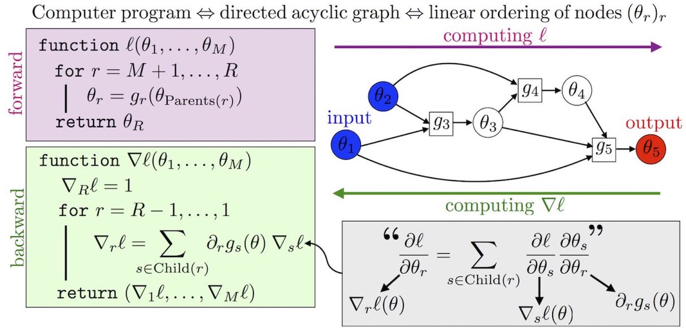
Backpropagation computations can be seen as message passing on the computational graph.
This procedure can be directly implemented using an ordered list and modular functions.

Backpropagation as Message Passing

Consider, standard backpropagation for computing $\mathbf{z}'$:
Not modular: $\mathbf{z}$ needs to know how it is used in the network for computing partial derivatives of $\mathbf{r}$, $\mathbf{s}$, and $\mathbf{t}$.

Backprop as Message Passing Continued...

Node receives messages from children, aggregates them to get its own error signal, then passes messages to parents.
Each message is a VJP

Modularity: each node needs to know how to compute its outgoing messages, i.e. the VJPs corresponding to each of its parents.
Implementation of $\mathbf{z}$ is agnostic to knowing where $\mathbf{z}'$ came from.

Backward Pass

The backwards pass is defined in core.py.
The argument $g$ is the error signal for the end node. This is always $\mathcal{L}' = 1$.


    def backward_pass(g, end_node):
      outgrads = {end_node : (g, False)}
      for node in toposort(end_node):
          outgrad = outgrads.pop(node)
          ingrads = node.vjp(outgrad[0])
          for parent, ingrad in zip(node.parents, ingrads):
              outgrads[parent] = add_outgrads(outgrads.get(parent), ingrad)
      return outgrad[0]

    def add_outgrads(prev_g, g):
      if prev_g is None:
        return g
      return prev_g + g

Backward Pass

grad is just a wrapper around make_vjp which builds the computation graph and feeds it to backward_pass.
grad itself is viewed as a VJP, if we treat $\bar{\mathcal{L}}$ as the $1 \times 1$ matrix with entry 1.

$\frac{\partial \mathcal{L}}{\partial \mathbf{w}} = \frac{\partial \mathcal{L}}{\partial \mathbf{w}}\bar{\mathcal{L}}$


    def make_vjp(fun, x):
      start_node = VJPNode.new_root()
      end_value, end_node =  trace(start_node, fun, x)
      if end_node is None:
          def vjp(g): return vspace(x).zeros()
      else:
          def vjp(g): return backward_pass(g, end_node)
      return vjp, end_value

    def grad(fun, argnum=0):
      def gradfun(*args, **kwargs):
        unary_fun = lambda x: fun(*subval(args, argnum, x), **kwargs)
        vjp, ans = make_vjp(unary_fun, args[argnum])
        return vjp(np.ones_like(ans))
      return gradfun

Automatic Differentiation Modes

Consider:

Forward-Mode Differentiation:
Reverse-Mode Differentiation:

Reverse-Mode AD

Matrix multiplication is associative: we can compute products in any order.
Computing products right-to-left avoids matrix-matrix products; only needs matrix-vector

Reverse Mode Automatic Differentiation

Forward-Mode AD

Computing products left-to-right avoids matrix-matrix products; only needs matrix-vector
Not implemented in Pytorch/Tensorflow

Higher-Order Derivatives

Hessian Matrix: second derivatives

$$\begin{equation}\frac{\partial^2 \mathcal{L}}{\partial \mathbf{x}^2}\end{equation} = \begin{bmatrix} \frac{\partial^2 \mathcal{L}}{\partial x_1^2} & \frac{\partial^2 \mathcal{L}}{\partial x_1\partial x_2} & \cdots & \frac{\partial^2 \mathcal{L}}{\partial x_1\partial x_n} \\ \frac{\partial^2 \mathcal{L}}{\partial x_2x_1} & \frac{\partial^2 \mathcal{L}}{\partial x^2_2} & \cdots & \frac{\partial^2 \mathcal{L}}{\partial x_2\partial x_n} \\ \vdots & \vdots & \ddots & \vdots \\ \frac{\partial^2 \mathcal{L}}{\partial x_1^2} & \frac{\partial^2 \mathcal{L}}{\partial x_1\partial x_2} & \cdots & \frac{\partial^2 \mathcal{L}}{\partial x_1\partial x_n} \end{bmatrix} $$

Hessian-vector multiply

$$\begin{equation}\frac{\partial^2 \mathcal{L}}{\partial \mathbf{x}^2_0}\mathbf{v}=\frac{\partial}{\partial \mathbf{x}_0}\left[\frac{\partial \mathcal{L}}{\partial \mathbf{x}_0}\cdot \mathbf{v}\right]\end{equation}$$