Normalizing Flows

CSE 891: Deep Learning

Vishnu Boddeti

Monday November 17, 2021

A Probabilistic Viewpoint

Goal: modeling $p_{data}$

Fully Observed Models

Transformation Models (likelihood free)

Latent Variable Models (observation noise)

Undirected Latent Variable Models (hidden factors)

Overview

How to fit a density model $p_{\theta}(\mathbf{x})$ with continuous $\mathbf{x}\in\mathbb{R}^n$
What do we want from this model?

Good fit to the training data (really, the underlying distribution!)
For new $\mathbf{x}$, ability to evaluate $p_{\theta}(\mathbf{x})$
Ability to sample from $p_{\theta}(\mathbf{x})$

And, ideally, a latent representation that is meaningful

Recap: Probability Density Models

$P(x\in[a,b]) = \int_a^b p(x)dx$

Recap: How to fit a density model?

Maximum Likelihood:
Equivalently:

Example: Mixture of Gaussians

\begin{equation} p_{\theta}(x) = \sum_{i=1}^k \pi_i\mathcal{N}(x_i;\mu_i,\sigma_i^2) \end{equation}

Parameters: means and variances of components, mixture weights $\theta = (\pi_1,\dots,\pi_k,\mu_1,\dots,\mu_k,\sigma_1,\dots,\sigma_k)$

How to fit a general density model?

How to ensure proper distribution? \begin{equation} \int_{\infty}^{\infty} p(x)dx = 1 \quad p_{\theta}(x) \geq 0 \forall x \end{equation}
How to sample?
Latent representation?

Flows: Main Idea

Generally: $\mathbf{z} \sim p_{Z}(\mathbf{z})$
Normalizing Flow: $\mathbf{z} \sim \mathcal{N}(0,1)$
Key questions:

How to train?
How to evaluate $p_{\theta}(x)$?
How to sample?

Flows: Training

\begin{equation}\max_{\theta}\sum_i \log p_{\theta}\left(x^{(i)}\right)\end{equation}

Need $f(\cdot)$ to be invertible and differentiable

Change of Variables Formula

Let $f^{-1}$ denote a differentiable, bijective mapping from space $\mathcal{Z}$ to space $\mathcal{X}$, i.e., it must be 1-to-1 and cover all of $\mathcal{X}$.
Since $f^{-1}$ defines a one-to-one correspondence between values $\mathbf{z} \in \mathcal{Z}$ and $\mathbf{x} \in \mathcal{X}$, we can think of it as a change-of-variables transformation.
Change-of-Variables Formula from probability theory. If $\mathbf{z} = f(\mathbf{x})$, then \begin{equation} p_{X}(\mathbf{x}) = p_Z(\mathbf{z})\left|det\left(\frac{\partial \mathbf{z}}{\partial \mathbf{x}}\right)\right| \nonumber \end{equation}

Intuition for the Jacobian term:

Flows: Training

\begin{equation}\max_{\theta}\sum_i \log p_{\theta}\left(x^{(i)}\right)\end{equation}

\begin{equation} \begin{aligned} \mathbf{z} &= f_{\theta}(\mathbf{x}) \\ p_{\theta}(\mathbf{x}) &= p_Z(\mathbf{z})\left|det\left(\frac{\partial \mathbf{z}}{\partial \mathbf{x}}\right)\right| \\ &= p_Z(f_{\theta}(\mathbf{x}))\left|det\left(\frac{\partial f_{\theta}(\mathbf{x})}{\partial \mathbf{x}}\right)\right| \\ \end{aligned} \end{equation}

\begin{equation}\max_{\theta}\sum_i \log p_{\theta}\left(x^{(i)}\right) = \max_{\theta}\sum_i \log p_Z(f_{\theta}(\mathbf{x}^{(i)})) + \log\left|det\left(\frac{\partial f_{\theta}(\mathbf{x})}{\partial \mathbf{x}}\right)\right|\end{equation}

Assuming we have an expression for $p_Z$, we can optimize this with Stochastic Gradient Descent

Flows: Sampling

Step 1: sample $\mathbf{z} \sim p_Z(\mathbf{z})$
Step 2: $\mathbf{x} = f^{-1}_{\theta}(\mathbf{z})$

Change of Variables Formula

Problems?

The mapping $f$ needs to be invertible, with an easy-to-compute inverse.
It needs to be differentiable, so that the Jacobian $\frac{\partial \mathbf{x}}{\partial \mathbf{z}}$ is defined.
We need to be able to compute the (log) determinant.

Example: Flow to Uniform $\mathbf{z}$

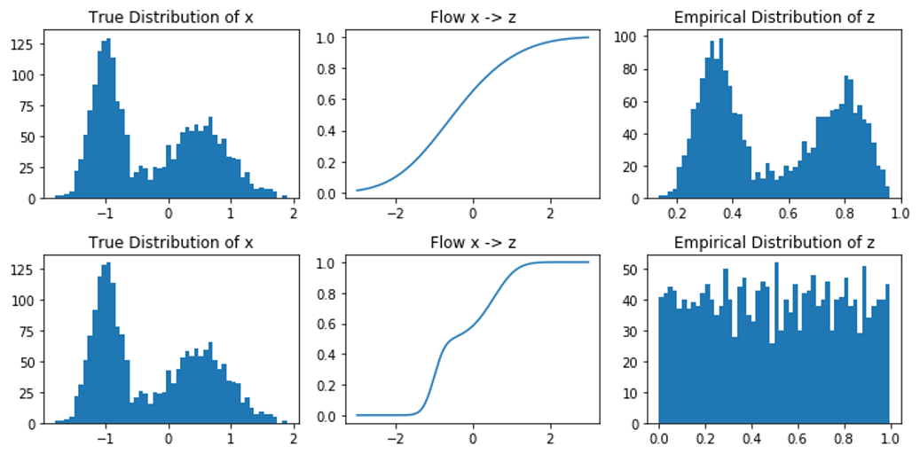
Example: Flow to Beta(5,5) $\mathbf{z}$

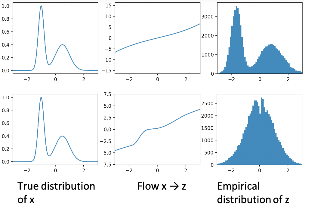
Example: Flow to Gaussian $\mathbf{z}$

2-D Autoregressive Flow

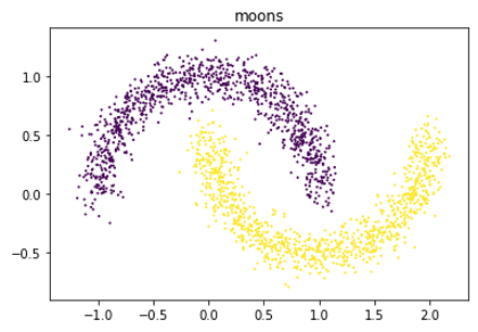
\begin{equation} \begin{aligned} x_1 &= z_1 = f_{\theta}(x_1) \\ x_2 &= z_2 = f_{\theta}(x_1,x_2) \\ \end{aligned} \end{equation}

2-D Autoregressive Flow: Two Moons

Architecture:

Base distribution: $Uniform[0,1]^2$
$x_1$: mixture of 5 Gaussians
$x_2$: mixture of 5 Gaussians, conditioned on $x_1$

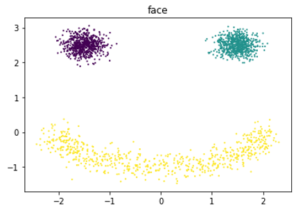
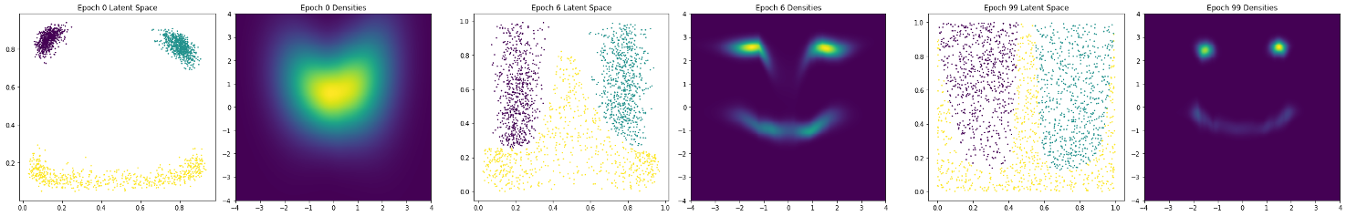
2-D Autoregressive Flow: Face

Architecture:

Base distribution: $Uniform[0,1]^2$
$x_1$: mixture of 5 Gaussians
$x_2$: mixture of 5 Gaussians, conditioned on $x_1$

High-Dimensional Data

Constructing Flows: Composition

Flows can be composed

\begin{equation} \begin{aligned} \mathbf{x} &\rightarrow f_1 \rightarrow f_2 \cdots \rightarrow f_k \rightarrow \mathbf{z} \\ \mathbf{z} &= f_k \circ \cdots \circ f_1(\mathbf{x}) \\ \mathbf{x} &= f_1^{-1} \circ \cdots \circ f_k^{-1}(\mathbf{z}) \\ \log p_{\theta}(\mathbf{x}) &= \log p_{\theta}(\mathbf{z}) + \sum_{i=1}^k\log \left|det\frac{\partial f_i}{\partial f_{i-1}}\right| \end{aligned} \end{equation}

Easy way to increase expressiveness

Affine Flows

Another name for affine flow: multivariate Gaussian.

Parameters: an invertible matrix $\mathbf{A}$ and a vector $\mathbf{b}$
$f(\mathbf{x}) = \mathbf{A}^{-1}(\mathbf{x}-\mathbf{b})$

Sampling: $\mathbf{x} = \mathbf{Az} + \mathbf{b}$, where $\mathbf{z} ~ \mathcal{N}(\mathbf{0}, \mathbf{I})$
Log likelihood is expensive when dimension is large.

The Jacobian of $f$ is $\mathbf{A}^{-1}$
Log likelihood involves calculating $det(\mathbf{A})$

Elementwise Flows

\begin{equation} f_{\theta}(x_1,x_2,\dots,x_n) = (f_{\theta}(x_1),\dots,f_{\theta}(x_1)) \end{equation}

Lots of freedom in elementwise flow

Can use elementwise affine functions or CDF flows.

The Jacobian is diagonal, so the determinant is easy to evaluate.

\begin{equation} \begin{aligned} \frac{\partial \mathbf{z}}{\partial \mathbf{x}} &= diag(f'_{\theta}(x_1), \dots, f'_{\theta}(x_d)) \\ det\left(\frac{\partial \mathbf{z}}{\partial \mathbf{x}}\right) &= \prod_{i=1}^d f'_{\theta}(x_i) \end{aligned} \end{equation}

Flows with Neural Networks?

Requirement: Invertible and Differentiable
Neural Network

If each layer is a flow, then sequencing of layers is also flow
Each layer: ReLU, Sigmoid, Tanh?

Reversible Blocks

Now let us define a reversible block which is invertible and has a tractable determinant.
Such blocks can be composed.

Inversion: $f^{-1} = f_1^{-1} \circ \dots \circ f_k^{-1}$
Determinants: $\left|\frac{\partial \mathbf{x}_k}{\partial \mathbf{z}}\right| = \left|\frac{\partial \mathbf{x}_k}{\partial \mathbf{x}_{k-1}}\right| \dots \left|\frac{\partial \mathbf{x}_2}{\partial \mathbf{x}_1}\right|\left|\frac{\partial \mathbf{x}_1}{\partial \mathbf{z}}\right|$

Reversible Blocks

Recall the residual blocks: \begin{equation} \mathbf{y} = \mathbf{x} + \mathcal{F}(\mathbf{x}) \nonumber \end{equation}
Reversible blocks are a variant of residual blocks. Divide the units into two groups, $\mathbf{x}_1$ and $\mathbf{x}_2$. \begin{eqnarray} \mathbf{y}_1 &=& \mathbf{x}_1 + \mathcal{F}(\mathbf{x}_2) \nonumber \\ \mathbf{y}_2 &=& \mathbf{x}_2 \nonumber \end{eqnarray}
Inverting the reversible block: \begin{eqnarray} \mathbf{x}_2 &=& \mathbf{y}_2 \nonumber \\ \mathbf{x}_1 &=& \mathbf{y}_1 - \mathcal{F}(\mathbf{x}_2) \nonumber \end{eqnarray}

Reversible Blocks

Composition of two reversible blocks, but with $\mathbf{x}_1$ and $\mathbf{x}_2$ swapped:

Forward: \begin{eqnarray} \mathbf{y}_1 &=& \mathbf{x}_1 + \mathcal{F}(\mathbf{x}_2) \nonumber\\ \mathbf{y}_2 &=& \mathbf{x}_2 + \mathcal{G}(\mathbf{y}_1) \nonumber \end{eqnarray}
Backward: \begin{eqnarray} \mathbf{x}_2 &=& \mathbf{y}_2 - \mathcal{G}(\mathbf{y}_1) \nonumber\\ \mathbf{x}_1 &=& \mathbf{y}_1 - \mathcal{F}(\mathbf{x}_2) \nonumber \end{eqnarray}

Volume Preservation

We still need to compute the log determinant of the Jacobian.

The Jacobian of the reversible block: \begin{eqnarray} \mathbf{y}_1 &=& \mathbf{x}_1 + \mathcal{F}(\mathbf{x}_2) \nonumber \\ \mathbf{y}_2 &=& \mathbf{x}_2 \nonumber \\ \frac{\partial \mathbf{y}}{\partial \mathbf{x}} &=& \begin{bmatrix} \mathbf{I} & \frac{\partial \mathcal{F}}{\partial \mathbf{x}_2} \\ \mathbf{0} & \mathbf{I} \end{bmatrix} \nonumber \end{eqnarray}

This is an upper triangular matrix. The determinant of an upper triangular matrix is the product of the diagonal entries, or in this case, 1.
Since the determinant is 1, the mapping is said to be volume preserving.

Nonlinear Independent Components Estimation

We just defined the reversible block.

Easy to invert by subtracting rather than adding the residual function.
The determinant of the Jacobian is 1.

Nonlinear Independent Components Estimation (NICE) trains a generator network which is a composition of lots of reversible blocks.
We can compute the likelihood function using the change-of-variables formula: \begin{equation} p_X(\mathbf{x}) = p_Z(\mathbf{z})\left|det\left(\frac{\partial \mathbf{x}}{\partial \mathbf{z}}\right)\right|^{-1} = p_Z(\mathbf{z}) \nonumber \end{equation}
We can train this model using maximum likelihood, i.e., given a dataset $\{\mathbf{x}^{(1)}, \dots, \mathbf{x}^{(N)}\}$, we maximize the likelihood: \begin{equation} \prod_{i=1}^N p_X(\mathbf{x}^{(i)}) = \prod_{i=1}^N p_Z(f^{-1}(\mathbf{x}^{(i)})) \nonumber \end{equation}

Nonlinear Independent Components Estimation

Likelihood:
Remember, $p_Z$ is a simple, fixed distribution (e.g. independent Gaussians)
Intuition: train the network such that $f(\cdot)$ maps each data point to a high-density region of the code vector space $\mathcal{Z}$.

Without constraints on $f(\cdot)$, it could map everything to 0, and this likelihood objective would make no sense.
But it cannot do this because it is volume preserving.

Nonlinear Independent Components Estimation

RealNVP

Reversible Model:

Forward Function: \begin{eqnarray} \mathbf{y}_1 &=& \mathbf{x}_1 \nonumber \\ \mathbf{y}_2 &=& \mathbf{x}_2 \odot \exp\left(\mathcal{F}_1(\mathbf{x}_1)\right) + \mathcal{F}_2(\mathbf{x}_1) \nonumber \end{eqnarray}
Inverse Function: \begin{eqnarray} \mathbf{x}_1 &=& \mathbf{y}_1 \nonumber \\ \mathbf{x}_2 &=& \left(\mathbf{y}_2 - \mathcal{F}_2(\mathbf{x}_1)\right) \odot \exp\left(-\mathcal{F}_1(\mathbf{x}_1)\right) \nonumber \end{eqnarray}

Jacobian: \begin{equation}\begin{bmatrix} \mathbf{I} & \mathbf{0} \\ \frac{\partial \mathbf{y}_2}{\partial \mathbf{x}_1} & diag(\exp(\mathcal{F}_1(\mathbf{x}_1)) \\ \end{bmatrix}\end{equation}