Variational Autoencoders
CSE 891: Deep Learning
Monday November 22, 2021
Latent Variable Model
- Goal: modeling $p_{data}$
- Autoregressive models
- All random variables are observed
- Latent Variable Models (LVMs)
- Some random variables are hidden - we do not get to observe


Why Latent Variable Models?
- Simpler, lower-dimensional representations of data often possible
- Latent variable models hold the promise of automatically identifying those hidden representations

Why Latent Variable Models?
- AR models are slow to sample because all pixels (observation dims) are assumed to be dependent on each other
- We can make part of observation space independent conditioned on some latent variables
- Latent variable models can have faster sampling by exploiting statistical patterns
Latent Variable Models
- Sometimes, it is possible to design a latent variable model with an understanding of the causal process that generates data
- In general, we do not know what are the latent variables and how they interact with observations
- Most popular models make little assumption about what are the latent variables
- Best way to specify latent variables is still an active area of research
Inferential Problems
- Evidence Estimation \begin{eqnarray} p(\mathbf{x}) = \int p(\mathbf{x},\mathbf{z})d\mathbf{z} \nonumber \end{eqnarray}
- Moment Computation \begin{eqnarray} \mathbb{E}[f(\mathbf{x})|\mathbf{z}] = \int f(\mathbf{x})p(\mathbf{x}|\mathbf{z})d\mathbf{x} \nonumber \end{eqnarray}
- Prediction \begin{eqnarray} p(\mathbf{x}_{t+1}) = \int p(\mathbf{x}_{t+1}|\mathbf{x}_t)p(\mathbf{x}_t)d\mathbf{x}_t \nonumber \end{eqnarray}
- Hypothesis Testing \begin{eqnarray} \mathcal{B} = \log p(\mathbf{x}|H_1) - \log p(\mathbf{x}|H_2) \nonumber \end{eqnarray}
Example Latent Variable Model
\begin{eqnarray} z &=& (z_1,z_2,\dots,z_K)\sim p(z;\beta)=\prod_{k=1}^K \beta_k^{z_k}(1-\beta)^{1-z_k} \\ x &=& (x_1,x_2,\dots,x_L)\sim p_{\theta}(x|z) \iff \mbox{Bernoulli}(x_i,DNN(z)) \end{eqnarray}
Latent Variable Model
- Sample: \begin{eqnarray} z &\sim& p(z) \\ x &\sim& p_{\theta}(x|z) \end{eqnarray}
- Evaluate Likelihood \begin{equation}p_{\theta}(x)=\sum_z p_Z(z)p_{\theta}(x|z)\end{equation}
- Train \begin{equation}\max_{\theta}\sum_i \log p_{\theta}(x^{(i)})=\sum_i\log\left(\sum_z p_Z(z)p_{\theta}(x^{(i)}|z)\right)\end{equation}
- Representation: $x \rightarrow z$
Training Latent Variable Model
- Objective: \begin{equation}\max_{\theta}\sum_i \log p_{\theta}(x^{(i)})=\sum_i\log\left(\sum_z p_Z(z)p_{\theta}(x^{(i)}|z)\right)\end{equation}
- Scenario 1: $z$ can only take on a small number of values $\rightarrow$ exact objective tractable
- Scenario 2: $z$ can only take on an impractical number of values $\rightarrow$ approximate
Bayesian Model Evidence

- Learning Principle: Model Evidence \[p(\mathbf{x}) = \int p(\mathbf{x},\mathbf{z})d\mathbf{z}\] \[\mathbf{x} = f(\mathbf{z})\]
- improve model evidence from data
- integral intractable in general
- idea: transform integral into expectation over simple known distribution
Importance Sampling
- $q(\mathbf{z}|\mathbf{x})>0$, when $f(\mathbf{z})p(\mathbf{z})\neq 0$
- Easy to sample from $q(\mathbf{z})$
\begin{eqnarray}
p(\mathbf{x}) &=& \int p(\mathbf{x}|\mathbf{z})p(\mathbf{z})d\mathbf{z} \nonumber \\
&=& \int p(\mathbf{x}|\mathbf{z})p(\mathbf{z})\frac{q(\mathbf{z}|\mathbf{x})}{q(\mathbf{z}|\mathbf{x})}d\mathbf{z} \nonumber \\
&=& \int p(\mathbf{x}|\mathbf{z})\frac{p(\mathbf{z})}{q(\mathbf{z}|\mathbf{x})}q(\mathbf{z}|\mathbf{x})d\mathbf{z} \nonumber \\
&& w^{(s)} = \frac{p(z)}{q(z|x)} \hspace{10pt} z^{(s)} \sim q(z|x) \nonumber \\
p(\mathbf{x}) &=& \frac{1}{S}\sum_{s} w^{(s)} p(\mathbf{x}|\mathbf{z}^{(s)}) \nonumber
\end{eqnarray}
Importance Sampling to Variational Inference
- Jensen's Inequality: \[\log \left(\int p(x)g(x)dx\right) \geq \int p(x)\log g(x)dx\]
- Variational Lower Bound: \[\mathbb{E}_{q(\mathbf{z}|\mathbf{x})}[\log p(\mathbf{x}|\mathbf{z})]-KL[q(\mathbf{z}|\mathbf{x})\|p(\mathbf{z})]\]
- Integral Problem: \begin{eqnarray} p(\mathbf{x}) &=& \int p(\mathbf{x}|\mathbf{z})p(\mathbf{z})d\mathbf{z} \nonumber \\ &=& \int p(\mathbf{x}|\mathbf{z})p(\mathbf{z})\frac{q(\mathbf{z}|\mathbf{x})}{q(\mathbf{z}|\mathbf{x})}d\mathbf{z} \nonumber \\ &=& \int p(\mathbf{x}|\mathbf{z})\frac{p(\mathbf{z})}{q(\mathbf{z}|\mathbf{x})}q(\mathbf{z}|\mathbf{x})d\mathbf{z} \nonumber \\ \log p(\mathbf{x}) &\geq& \int q(\mathbf{z}|\mathbf{x})\log\left(p(\mathbf{x}|\mathbf{z})\frac{p(\mathbf{z})}{q(\mathbf{z}|\mathbf{x})}\right) \nonumber \\ &=& \int q(\mathbf{z}|\mathbf{x})\log p(\mathbf{x}|\mathbf{z}) - \int q(\mathbf{z}|\mathbf{x})\log \frac{q(\mathbf{z}|\mathbf{x})}{p(\mathbf{z})} \nonumber \end{eqnarray}
Variational Free Energy
\begin{equation} \mathcal{F}(\mathbf{x},q) = \underbrace{\mathbb{E}_{q(\mathbf{z}|\mathbf{x})}[\log p(\mathbf{x}|\mathbf{z})]}_{\text{Reconstruction}}-\underbrace{KL[q(\mathbf{z}|\mathbf{x})\|p(\mathbf{z})]}_{\text{Penalty}} \nonumber \end{equation}
- Interpreting the Lower Bound:
- Approximate posterior distribution $q(\mathbf{z}|\mathbf{x})$: Best match to true posterior $p(\mathbf{z}|\mathbf{x})$, one of the unknown inferential quantities of interest to us.
- Reconstruction Cost: The expected log-likelihood measures how well samples from $q(\mathbf{z}|\mathbf{x})$ are able to explain the data $\mathbf{x}$.
- Penalty: Ensures that the explanation of the data $q(\mathbf{z}|\mathbf{x})$ doesn't deviate too far from your beliefs $p(\mathbf{z})$. A mechanism for realizing Ockham's razor.
Other Families of Variational Bounds
Variational Free Energy\begin{equation} \mathcal{F}(\mathbf{x},q) = \mathbb{E}_{q(\mathbf{z}|\mathbf{x})}[\log p(\mathbf{x}|\mathbf{z})]-KL[q(\mathbf{z}|\mathbf{x})\|p(\mathbf{z})] \nonumber \end{equation}Multi-Sample Variational Objective
\begin{equation} \mathcal{F}(\mathbf{x},q) = \mathbb{E}_{q(\mathbf{z}|\mathbf{x})}\left[\log \frac{1}{S}\sum_{S} \frac{p(\mathbf{z})}{q(\mathbf{z}|\mathbf{x})}p(\mathbf{x}|\mathbf{z})\right] \nonumber \end{equation}Renyi Divergence
\begin{equation} \mathcal{F}(\mathbf{x},q) = \frac{1}{1-\alpha}\mathbb{E}_{q(\mathbf{z}|\mathbf{x})}\left[\left(\log \frac{1}{S}\sum_{S} \frac{p(\mathbf{z})}{q(\mathbf{z}|\mathbf{x})}p(\mathbf{x}|\mathbf{z})\right)^{1-\alpha}\right] \nonumber \end{equation}
Learning: Variational EM
\begin{equation} \mathcal{F}(\mathbf{x},q) = \mathbb{E}_{q(\mathbf{z}|\mathbf{x})}[\log p(\mathbf{x}|\mathbf{z})]-KL[q(\mathbf{z}|\mathbf{x})\|p(\mathbf{z})] \nonumber \end{equation}
- Alternating Optimization
- Repeat:
- E-Step: $\phi \propto \nabla_{\phi}\mathcal{F}(\mathbf{x},q)$ (Variational params)
- M-Step: $\theta \propto \nabla_{\theta}\mathcal{F}(\mathbf{x},q)$ (Model params)

Stochastic Approximation
\begin{equation} \mathcal{F}(\mathbf{x},q) = \mathbb{E}_{q(\mathbf{z}|\mathbf{x})}[\log p(\mathbf{x}|\mathbf{z})]-KL[q(\mathbf{z}|\mathbf{x})\|p(\mathbf{z})] \nonumber \end{equation}
- Optimize using a stochastic gradient based on a mini-batch of data
- $N$ is a mini-batch sampled with replacement from the full dataset.
- E-Step (compute $q$): Inference \begin{eqnarray} \text{For } n&=&1,\dots,N \nonumber \\ && \phi \propto \nabla_{\phi} \mathbb{E}_{q_{\phi}(z)}[\log p(\mathbf{x}_n|\mathbf{z}_n)]-KL[q(\mathbf{z}_n|\mathbf{x}_n)\|p(\mathbf{z})] \nonumber \end{eqnarray}
- M-Step: Parameter Learning \[\theta \propto \frac{1}{N}\sum_{n} \mathbb{E}_{q_{\phi}(z)}[\nabla_{\theta}\log p_{\theta}(\mathbf{x}_n|\mathbf{z}_n)]\]
Memoryless Inference
\begin{equation} \mathcal{F}(\mathbf{x},q) = \mathbb{E}_{q(\mathbf{z}|\mathbf{x})}[\log p(\mathbf{x}|\mathbf{z})]-KL[q(\mathbf{z}|\mathbf{x})\|p(\mathbf{z})] \nonumber \end{equation}
- E-step does not reuse any previous computation.
- Memoryless: Any inference computations are discarded after the M-step update.
- E-Step (compute $q$): Inference \begin{eqnarray} \text{For } n&=&1,\dots,N \nonumber \\ && \phi \propto \nabla_{\phi} \mathbb{E}_{q_{\phi}(z)}[\log p(\mathbf{x}_n|\mathbf{z}_n)]-KL[q(\mathbf{z}_n|\mathbf{x}_n)\|p(\mathbf{z})] \nonumber \end{eqnarray}
- M-Step: Parameter Learning \[\theta \propto \frac{1}{N}\sum_{n} \mathbb{E}_{q_{\phi}(z)}[\nabla_{\theta}\log p_{\theta}(\mathbf{x}_n|\mathbf{z}_n)]\]
Amortized Inference
- Instead of solving E-step for every observation, amortize using a model.
- Inference Network: $q$ is an encoder, an inverse model, recognition model.
- Parameters of $q$ are now a set of global parameters used for inference of all the data points, both test and train.
- Amortize (spread) the cost of inference over all data.
- Joint optimization of variational and model parameters.

Amortized Variational Inference
\begin{equation} \mathcal{F}(\mathbf{x},q) = \mathbb{E}_{q(\mathbf{z}|\mathbf{x})}[\log p(\mathbf{x}|\mathbf{z})]-KL[q(\mathbf{z}|\mathbf{x})\|p(\mathbf{z})] \nonumber \end{equation}
- Variational Auto-Encoder: Specific combination of variational inference in latent variable models using inference networks
- Model (Decoder): likelihood $p(\mathbf{x}|\mathbf{z})$
- Inference (Encoder): variational distribution $q(\mathbf{z}|\mathbf{x})$
- Transforms an auto-encoder into a generative model.


Latent Gaussian VAE
\begin{eqnarray} p(\mathbf{z}) &=& \mathcal{N}(\mathbf{0},\mathbf{I}) \nonumber \\ p_{\theta}(\mathbf{x}|\mathbf{z}) &=& \mathcal{N}(\mathbf{\mu}_{\theta}(\mathbf{z}),\mathbf{\Sigma}_{\theta}(\mathbf{z})) \nonumber \\ q_{\phi}(\mathbf{z}|\mathbf{x}) &=& \mathcal{N}(\mathbf{\mu}_{\phi}(\mathbf{x}),\mathbf{\Sigma}_{\phi}(\mathbf{x})) \nonumber \end{eqnarray}

$KL(p\|q)$ vs $KL(q\|p)$

Reverse KL: Zero-Forcing/Mode-Seeking
Forward KL: Mass-Covering/Mean-Seeking
Variational Auto-Encoders in General
\begin{equation} \mathcal{F}(q) = \mathbb{E}_{q_{\phi}(\mathbf{z}|\mathbf{x})}[\log p_{\theta}(\mathbf{x}|\mathbf{z})]-KL[q_{\phi}(\mathbf{z}|\mathbf{x})\|p(\mathbf{z})] \nonumber \end{equation}
- Design Choices:
- Prior on latent variables: continuous, discrete, Gaussian, Bernoulli, mixture
- Likelihood Function: iid (static), sequential, temporal, spatial
- Approximating Posterior: distribution, sequential, spatial
- Scalability and Ease of Implementation:
- stochastic gradient estimation
- stochastic gradient descent (and variants)
Minimum Description Length
\begin{equation} \mathcal{F}(\mathbf{x},q) = \underbrace{\mathbb{E}_{q(\mathbf{z}|\mathbf{x})}[\log p(\mathbf{x}|\mathbf{z})]}_{\text{Data code-length}}-\underbrace{KL[q(\mathbf{z}|\mathbf{x})\|p(\mathbf{z})]}_{\text{Hypothesis code}} \nonumber \end{equation}
- Compressibility: Regularity in our data can be explained with latent variables.
- Inference is a problem of compression.
- Minimum Description Length (MDL):
- we must find the ideal shortest message of our data $\mathbf{x}$: marginal likelihood.
- Must introduce an approximation to the ideal message.
Learning: Stochastic Backpropagation
Common gradient problem\begin{equation} \nabla_{\phi}\mathbb{E}_{q_{\phi}(\mathbf{z})}[f_{\theta}(\mathbf{z})] = \nabla \int q_{\phi}(\mathbf{z})f_{\theta}(\mathbf{z})d\mathbf{z} \nonumber \end{equation}


\[\mathbf{z} \sim q_{\phi}(\mathbf{x})\] \[\mathbf{z} = g(\epsilon,\phi)\] \[\epsilon \sim p(\epsilon)\]
Generating Complex Distributions
- Generating complex distributions from simple distributions.
- Substitute random variable by deterministic function of simpler random variable.
| $\mathcal{N}(0,1)$ | $\epsilon \sim [0,1]$ | $\sqrt{ln\left(\frac{1}{\epsilon_1}\right)}\cos(2\pi\epsilon_2)$ |
| $\mathcal{N}(\mathbf{\mu},\mathbf{RR}^T)$ | $\epsilon \sim \mathcal{N}(\mathbf{0},\mathbf{I})$ | $\mu + \mathbf{R}\mathbf{\epsilon}$ |
| $\exp(-x); x > 0$ | $\epsilon \sim [0,1]$ | $ln\left(\frac{1}{\epsilon}\right)$ |
| $\frac{1}{\pi(1+x^2)}$ | $\epsilon \sim [0,1]$ | $tan(\pi\epsilon)$ |
| $\exp(-|x|)$ | $\epsilon \sim [0,1]$ | $ln\left(\frac{\epsilon_1}{\epsilon_2}\right)$ |
Implementing Variational Algorithms
Ideally want probabilistic programming using variational inference. Variational inference turns integration into optimization.
- Differentiation: PyTorch, TensforFlow
- Stochastic gradient descent and other preconditioned optimization
- Same code can run on GPUs and distributed clusters
- Probabilistic models are modular and can be easily combined

Visualizing Latent Space


Interpolating Latent Space

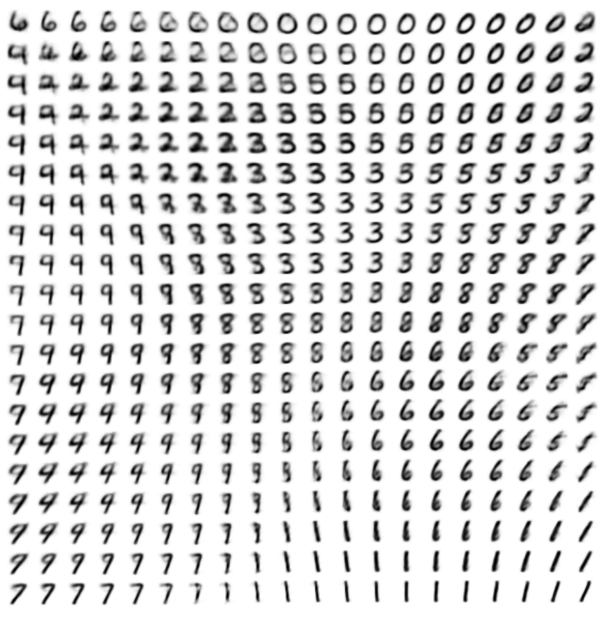
Interpolating Latent Space
VQ-VAE
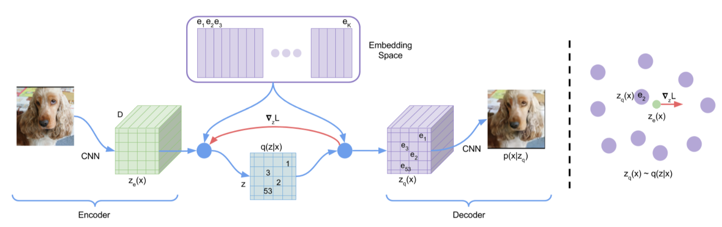 \begin{equation}
L = \log p(x|z_q(x)) + \|sg[z_e(x)]-e\|_2^2 + \beta\|z_e(x)-sg[e]\|_2^2
\end{equation}
\begin{equation}
L = \log p(x|z_q(x)) + \|sg[z_e(x)]-e\|_2^2 + \beta\|z_e(x)-sg[e]\|_2^2
\end{equation}
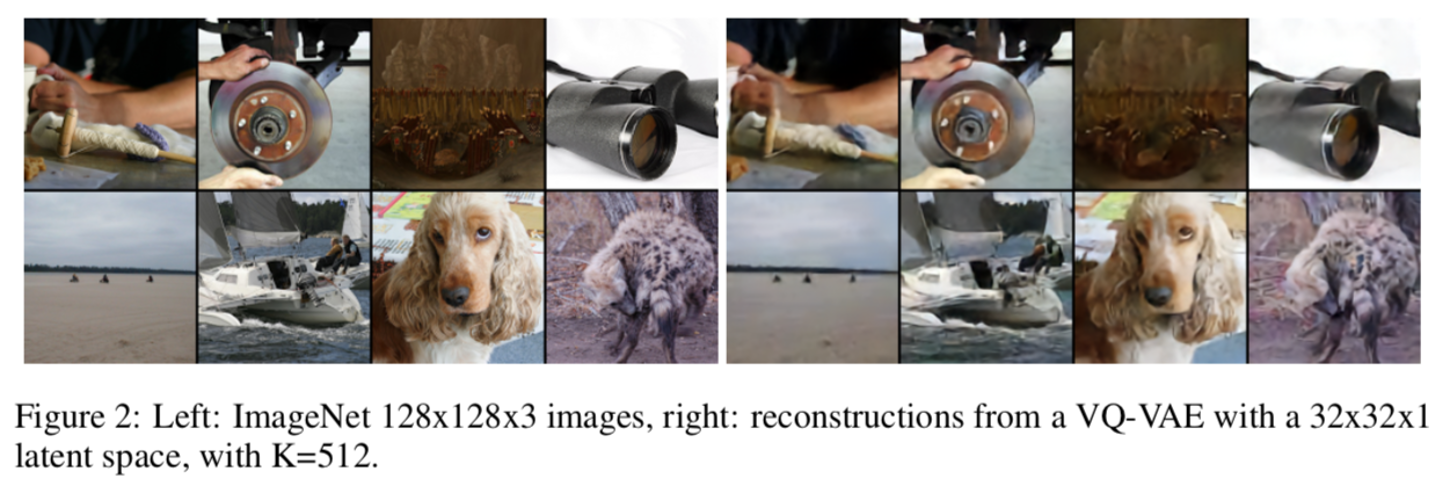
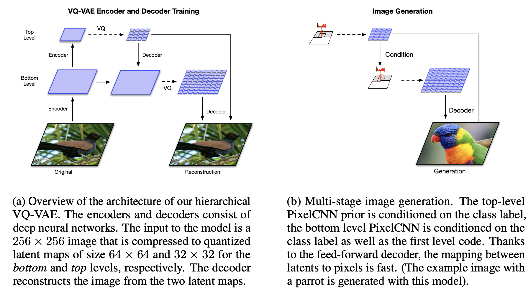
VQ-VAE
VQ-VAE-2
Learning Disentangled Representations
\begin{equation} \mathcal{F}(\mathbf{x},q) = \mathbb{E}_{q(\mathbf{z}|\mathbf{x})}[\log p(\mathbf{x}|\mathbf{z})]-\beta KL[q(\mathbf{z}|\mathbf{x})\|p(\mathbf{z})] \nonumber \end{equation}


Learning Disentangled Representations
