Deep Reinforcement Learning

Deep Reinforcement Learning - I

CSE 891: Deep Learning

Vishnu Boddeti

Monday December 01, 2021

Overview

Most of this course was about supervised and unsupervised learning.
We will look at another machine learning topic, Reinforcement Learning.

Conceptually, somewhere in between supervised and unsupervised learning.
An agent acts in an environment and receives a reward signal.

Today: policy gradient (directly do SGD over a stochastic policy using trial-and-error)

Reinforcement Learning

An agent interacts with an environment.
In each time step $t$,

the agent receives observations which give it information about the state $\mathbf{s}_t$ (e.g. positions of the ball and paddle)
the agent picks an action $\mathbf{a}_t$ which affects the state

The agent periodically receives a reward $r(\mathbf{s}_t, \mathbf{a}_t)$, which depends on the state and action
The agent wants to learn a policy $\pi_{\mathbf{\theta}}(\mathbf{a}_t | \mathbf{s}_t)$

Distribution over actions depending on the current state and parameters $\mathbf{\theta}$

Markov Decision Processes

The environment is represented as a Markov Decision Process $\mathcal{M}$.
Markov assumption: all relevant information is encapsulated in the current state; i.e. the policy, reward, and transitions are all independent of past states given the current state

Components of an MDP:

initial state distribution $p(\mathbf{s}_0)$
policy $\pi_{\mathbf{\theta}}(\mathbf{a}_t|\mathbf{s}_t)$
transition distribution $p(\mathbf{s}_{t+1}|\mathbf{s}_t, \mathbf{a}_t)$
reward function $r(\mathbf{s}_t, \mathbf{a}_t)$

Markov Decision Processes

Goal: Find the optimal policy $\pi^*$ that maximizes (discounted) sum of rewards.
Problem: Lots of randomness in terms of initial state, transition probabilities and rewards.
Assume a fully observable environment, i.e. $\mathbf{s}_t$ can be observed directly
Rollout, or trajectory $\tau = (\mathbf{s}_0, \mathbf{a}_0, \mathbf{s}_1, \mathbf{a}_1, \dots, \mathbf{s}_T, \mathbf{a}_T )$
Probability of rollout: \begin{equation} \begin{aligned} p(\tau) = p(\mathbf{s}_0)\pi_{\mathbf{\theta}}(\mathbf{a}_0|\mathbf{s}_0)p(\mathbf{s}_1|\mathbf{s}_0, \mathbf{a}_0)\pi_{\mathbf{\theta}}(\mathbf{a}_1|\mathbf{s}_1) \cdots p(\mathbf{s}_T|\mathbf{s}_{T-1},\mathbf{a}_{T-1})\pi_{\mathbf{\theta}}(\mathbf{a}_T|\mathbf{s}_T) \nonumber \end{aligned} \end{equation}

Markov Decision Processes

Continuous control tasks, e.g., teaching a simulated ant to walk.

State: positions, angles, and velocities of the joints
Action: apply forces to the joints
Reward: distance from starting point
Policy: output of an ordinary MLP, using the state as input

Markov Decision Processes

Return for a rollout: $r(\tau) = \sum_{t=0}^T r(\mathbf{s}_t, \mathbf{a}_t)$

Here we consider a finite horizon $T$; we will look at infinite horizon case later.

Goal: maximize the expected return, $R = \mathbb{E}_{p(\tau)}[r(\tau)]$
The expectation is over both the dynamics of the environment as well as the policy, but we can only control the policy.
The stochastic policy is important, since it makes $R$ a continuous function of the policy parameters.

Reward functions and dynamics are often discontinuous (e.g. collisions)

Markov Decision Processes

REINFORCE

REINFORCE is an elegant algorithm for maximizing the expected return $R=\mathbb{E}_{p(\tau)}[r(\tau)]$
Intuition: trial and error

Sample a rollout $\tau$. If you get a high reward, try to make it more likely. If you get a low reward, try to make it less likely.

Interestingly, this can be seen as stochastic gradient ascent on R.

REINFORCE

Gradient of the expected return:
Derivative formula for $\log$: \begin{equation} \frac{\partial}{\partial \mathbf{\theta}}\log p(\tau) = \frac{\frac{\partial}{\partial \mathbf{\theta}}p(\tau)}{p(\tau)} \Rightarrow \frac{\partial}{\partial \mathbf{\theta}}p(\tau) = p(\tau)\frac{\partial}{\partial \mathbf{\theta}}\log p(\tau) \nonumber \end{equation}
Compute stochastic estimates of this expectation by sampling rollouts.

REINFORCE

If you get a large reward, make the rollout more likely. If you get a small reward, make it less likely.
REINFORCE gradient: \begin{equation} \begin{aligned} \frac{\partial}{\partial \mathbf{\theta}} \log p(\tau) &= \frac{\partial}{\partial \mathbf{\theta}}\log \left[p(\mathbf{s}_0)\prod_{t=1}^T\pi_{\mathbf{\theta}}(\mathbf{a}_t|\mathbf{s}_t)\prod_{t=1}^Tp(\mathbf{s}_t|\mathbf{s}_{t-1},\mathbf{a}_{t-1})\right] \\ &= \frac{\partial}{\partial \mathbf{\theta}} \log\prod_{t=1}^T \pi_{\mathbf{\theta}}(\mathbf{a}_t|\mathbf{s}_t) \\ &= \log\prod_{t=1}^T \frac{\partial}{\partial \mathbf{\theta}}\pi_{\mathbf{\theta}}(\mathbf{a}_t|\mathbf{s}_t) \end{aligned} \end{equation}
REINFORCE tries to make all the actions more likely or less likely, depending on the reward, i.e., it does not do credit assignment.

REINFORCE

Repeat Forever:

Sample a rollout $\tau=(\mathbf{s}_0,\mathbf{a}_0,\mathbf{s}_1,\mathbf{a}_1,\dots,\mathbf{s}_T,\mathbf{a}_T)$

$r(\tau) \leftarrow \sum_{t=0}^T r(\mathbf{s}_t, \mathbf{a}_t)$

for $k = 0,\dots,T$ do

$\quad \mathbf{\theta} \leftarrow \mathbf{\theta} + \alpha r(\tau)\frac{\partial}{\partial \mathbf{\theta}}\log \pi_{\mathbf{\theta}}(\mathbf{a}_k|\mathbf{s}_k)$

end for

Observation: Actions should only be reinforced based on future rewards. Actions cannot influence past rewards.

REINFORCE

Repeat Forever:

Sample a rollout $\tau=(\mathbf{s}_0,\mathbf{a}_0,\mathbf{s}_1,\mathbf{a}_1,\dots,\mathbf{s}_T,\mathbf{a}_T)$

for $k = 0,\dots,T$ do

$\quad r(\tau)_t \leftarrow \sum_{k=t}^T r(\mathbf{s}_t, \mathbf{a}_t)$

$\mathbf{\theta} \leftarrow \mathbf{\theta} + \alpha r(\tau)_t\frac{\partial}{\partial \mathbf{\theta}}\log \pi_{\mathbf{\theta}}(\mathbf{a}_k|\mathbf{s}_k)$

end for

You can show that this still gives unbiased gradient estimates.

Optimizing Discontinuous Objectives

Edge case of RL: handwritten digit classification, but maximizing accuracy (or minimizing 0–1 loss)
Gradient descent completely fails if the cost function is discontinuous:

Supervised learning solution: use a surrogate loss function, e.g. logistic-cross-entropy
RL formulation: in each episode, the agent is shown an image, guesses a digit class, and receives a reward of 1 if it is correct or 0 if it is wrong.
In practice, we would never actually do it this way, but it gives us an interesting comparison with backprop.

Optimizing Discontinuous Objectives

RL Formulation:

one step at a time
state $\mathbf{x}$: an image
action $\mathbf{a}$: a digit class
reward $r(\mathbf{s},\mathbf{a})$: 1 if correct and 0 if wrong
policy $\pi_{\mathbf{\theta}}(\mathbf{a}|\mathbf{s})$: a distribution over classes

policy network: can be implemented through a MLP with softmax outputs

Optimizing Discontinuous Objectives

Let $t$ the integer target, $\mathbf{t}_k$ the target one-hot representation, $\mathbf{z}_k$ denote the logits, and $\mathbf{y}_k$ denote the softmax output.
To use REINFORCE, we sample $\mathbf{a} \sim \pi_{\mathbf{\theta}}(\cdot | \mathbf{x})$ and apply: \begin{equation} \begin{aligned} \mathbf{\theta} &\leftarrow \mathbf{\theta} + \alpha r(\mathbf{a},\mathbf{t})\frac{\partial}{\partial \mathbf{\theta}}\log \pi_{\theta}(\mathbf{a}|\mathbf{x}) \\ &= \mathbf{\theta} + \alpha r(\mathbf{a},\mathbf{t})\frac{\partial}{\partial \mathbf{\theta}} \log y_{a} \\ &= \mathbf{\theta} + \alpha r(\mathbf{a},\mathbf{t})\sum_{k=1}(a_k - y_k)\frac{\partial}{\partial \mathbf{\theta}} z_k \end{aligned} \end{equation}
Logistic regression SGD update: \begin{equation} \begin{aligned} \mathbf{\theta} &\leftarrow \mathbf{\theta} + \alpha \frac{\partial}{\partial \mathbf{\theta}} \log y_t\\ &= \mathbf{\theta} + \alpha \sum_{k=1}(t_k-y_k)\frac{\partial}{\partial \mathbf{\theta}} z_k \end{aligned} \end{equation}

Reward Functions

Update rule: \[\mathbf{\theta} \leftarrow \mathbf{\theta} + \alpha r(\mathbf{a},\mathbf{t})\frac{\partial}{\partial \mathbf{\theta}}\log \pi_{\theta}(\mathbf{a}|\mathbf{x})\]
A constant offset can be added to the reward to obtain an equivalent optimization problem.
Behavior if $r = 0$ for wrong answers and $r = 1$ for correct answers

wrong: do nothing, correct: make the action more likely

If $r = 10$ for wrong answers and $r = 11$ for correct answers

wrong: make the action more likely, correct: make the action even more likely

If $r = -10$ for wrong answers and $r = -9$ for correct answers

wrong: make the action less likely, correct: make the action less likely, but not as much

Reward Functions

Problem: REINFORCE update depends on arbitrary constant factors added to the reward.
Observation: we can subtract a baseline $b$ from the reward without biasing the gradient. \begin{equation} \begin{aligned} \mathbb{E}_{p(\tau)}\left[(r(\tau)-b)\frac{\partial}{\partial\mathbf{\theta}}\log p(\tau)\right] &= \mathbb{E}_{p(\tau)}\left[r(\tau)\frac{\partial}{\partial\mathbf{\theta}}\log p(\tau)\right] - b\mathbb{E}_{p(\tau)}\left[\frac{\partial}{\partial\mathbf{\theta}}\log p(\tau)\right] \\ &= \mathbb{E}_{p(\tau)}\left[r(\tau)\frac{\partial}{\partial\mathbf{\theta}}\log p(\tau)\right] - b\sum_{\tau}p(\tau)\frac{\partial}{\partial\mathbf{\theta}}\log p(\tau) \\ &= \mathbb{E}_{p(\tau)}\left[r(\tau)\frac{\partial}{\partial\mathbf{\theta}}\log p(\tau)\right] - b\sum_{\tau}\frac{\partial}{\partial\mathbf{\theta}}p(\tau) \\ &= \mathbb{E}_{p(\tau)}\left[r(\tau)\frac{\partial}{\partial\mathbf{\theta}}\log p(\tau)\right] - 0 \end{aligned} \end{equation}
Pick a baseline $b$ such that good rewards are positive and bad ones are negative.
$\mathbb{E}[r(\tau)]$ is a good choice of baseline, but cannot always be computed easily. Lots of research on trying to approximate it.

Getting Policy Gradient to Work

Evaluate each action using only future rewards, since it has no influence on past rewards. It can be shown this gives unbiased gradients.
Natural policy gradient corrects for the geometry of the space of policies, preventing the policy from changing too quickly.
Rather than use the actual return, evaluate actions based on estimates of future returns. This is a class of methods known as actor-critic.
Trust region policy optimization (TRPO) and proximal policy optimization (PPO) are modern policy gradient algorithms which are very effective for continuous control problems.

Backpropagation vs REINFORCE

Backpropagation: Does credit assignment – it tells you exactly which activations and parameters should be adjusted upwards or downwards to decrease the loss on some training example.
REINFORCE: Does not do credit assignment. If a rollout happens to be good, all the actions get reinforced, even if some of them were bad.
Reinforcing all the actions as a group leads to random walk behavior.

Why Policy Gradients

Can handle discontinuous cost functions.
Does not need an explicit model of the environment, i.e. environment rewards and dynamics are treated as black boxes.

Policy gradient is an example of model-free reinforcement learning, since the agent doesn’t try to fit a model of the environment.
Almost everyone thinks model-based approaches are needed for AI, but nobody has a clue how to get it to work.

Evolution Strategies

REINFORCE can handle discontinuous dynamics and reward functions, but needs a differentiable network since it computes $\frac{\partial}{\partial \mathbf{\theta}}\log \pi_{\theta}(\mathbf{a}_t|\mathbf{s}_t)$.
Evolution strategies (ES) take the policy gradient idea a step further, and avoid backprop entirely.
ES can use deterministic policies. It randomizes over the choice of policy rather than over the choice of actions.

sample a random policy from a distribution $p_{\eta}(\mathbf{\theta})$ parameterized by $\eta$ and apply the policy gradient trick \begin{equation} \frac{\partial}{\partial \eta}\mathbb{E}_{\mathbf{\theta}\sim p{\eta}}[r(\tau(\mathbf{\theta}))] = \mathbb{E}_{\mathbf{\theta}\sim p{\eta}}\left[r(\tau(\mathbf{\theta}))\frac{\partial}{\partial \eta}\log p_{\eta}(\mathbf{\theta})\right] \nonumber \end{equation}

The policy network itself can be discontinuous.

Evolution Strategies

Salimans et. al. Evolution Strategies as a Scalable Alternative to Reinforcement Learning, arXiv:1703.03864

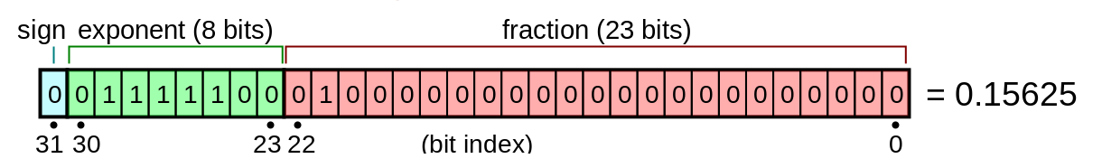
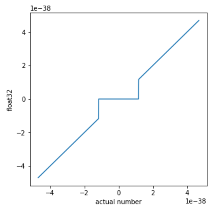
Evolution Strategies: IEEE Floating Point

The IEEE floating point standard is nonlinear, since small enough numbers get truncated to zero.

This acts as a discontinuous activation function, which ES is able to handle.
ES was able to train a good MNIST classifier using a "linear" activation function.