Convolutional Neural Networks
CSE 891: Deep Learning
Overview
- So far in the course,
- our NN layers do not respect the spatial structure of images.
- Solution: Define new computational nodes that operate on images.
- Key Idea:
- local connectivity
- parameter sharing
Components of Modern Network
- Fully Connected Layers
- Activation Functions
- FConvolutional Layers
- Pooling Layers
- Normalization Layers
Convolution Layers
Fully Connected Layer

- $32\times 32 \times 3$ image -> stretched to $3072 \times 1$
Convolution Layer

- $3 \times I \times I$ images preserves spatial structure
- Convolve the filter with the image i.e., "slide over the image spatially, computing dot products."
- Filters always extend the full depth of the input volume.
Convolution Layer

- 1 number: the result of taking a dot product between the filter and a small $3\times W \times W$ chunk of the image i.e., $\mathbf{w}^T\mathbf{x} + \mathbf{b}$
Convolution Layer

Convolution Layer

Stacking Convolutions


- What happens if we stack two convolutional layers?
- Problem: We get another convolution
- Solution: Add a non-linear layer between any two linear layers
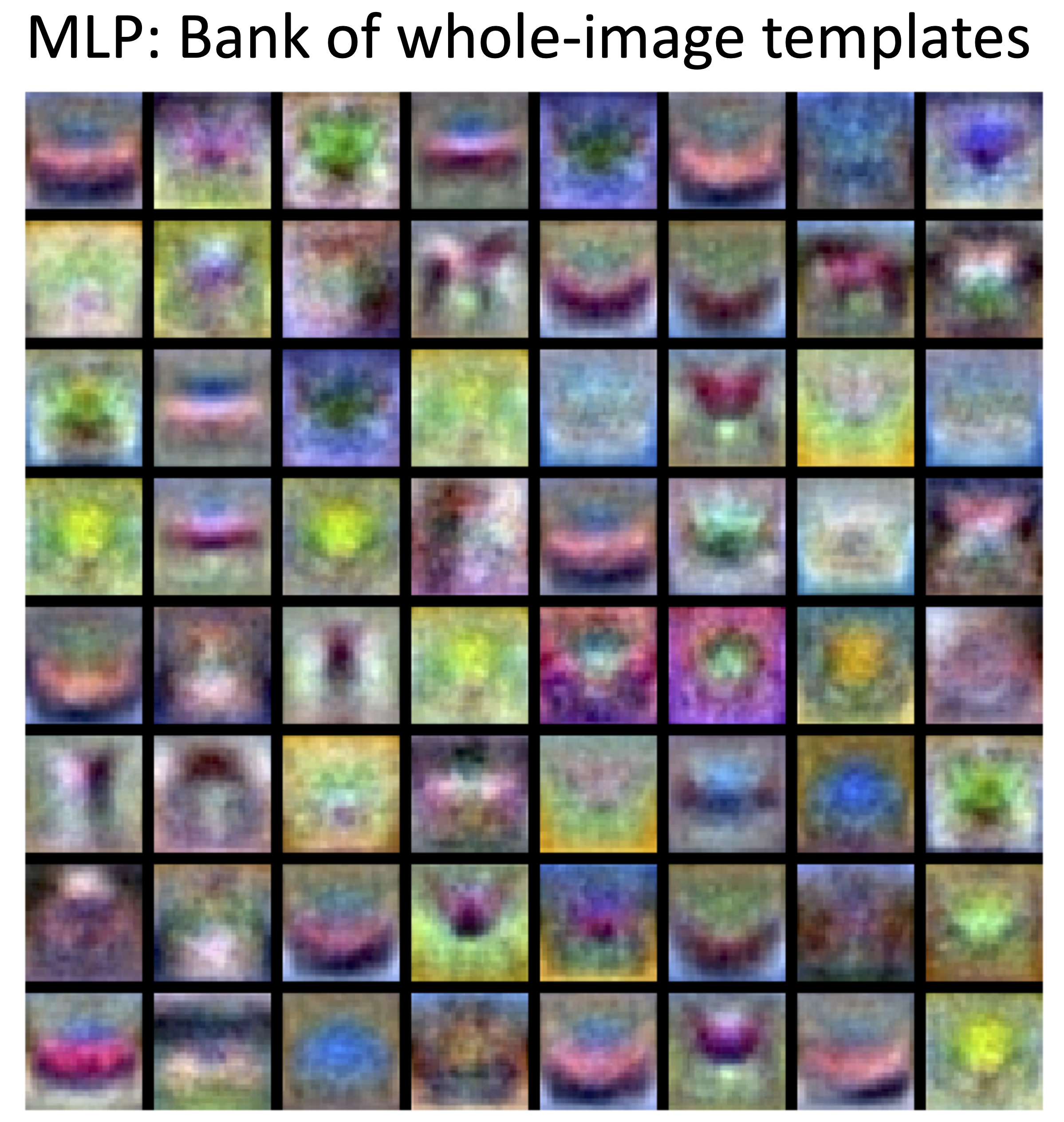
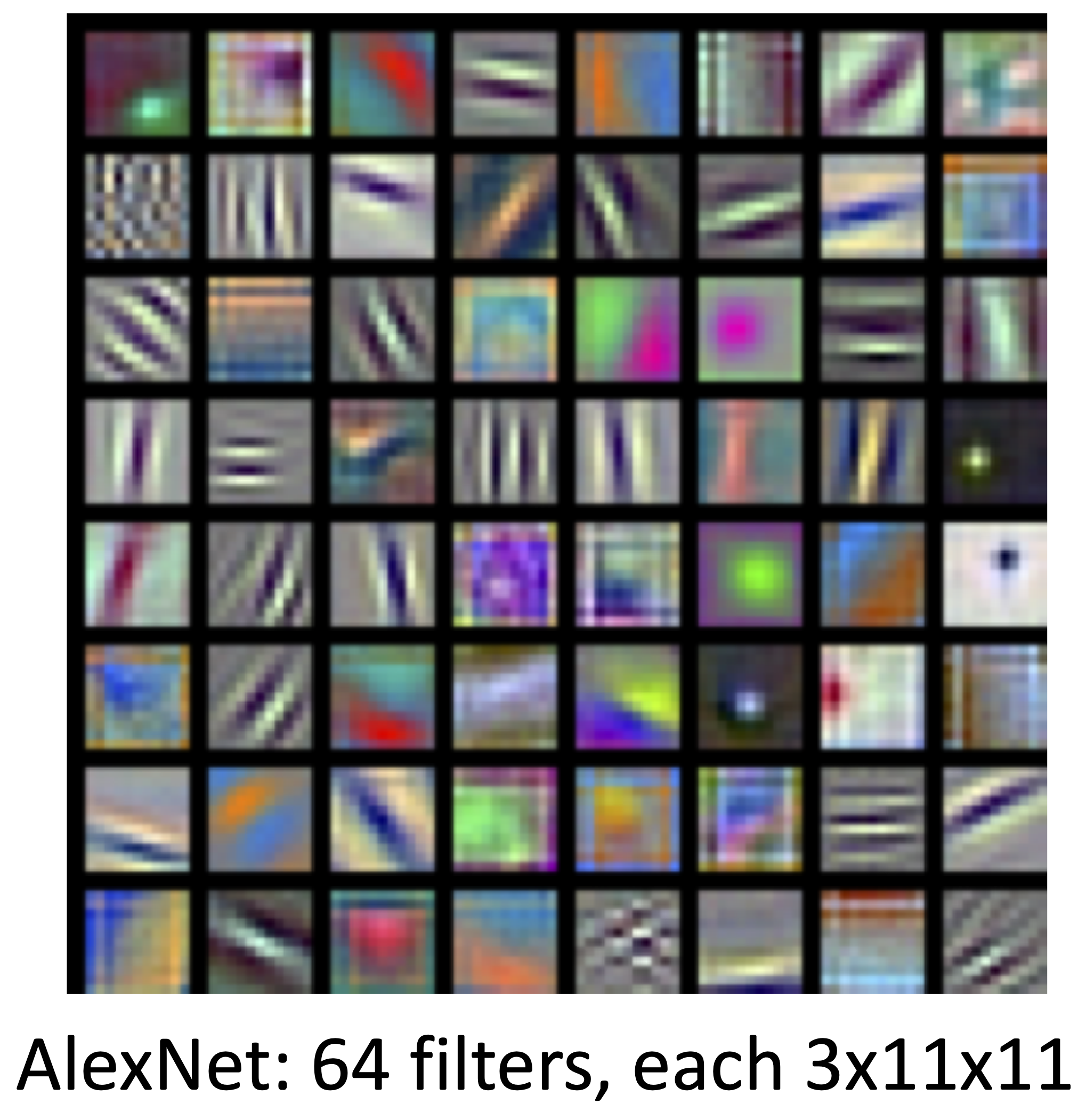
Learned Convolution Filters

Strided Convolution
- Input: $7\times 7$
- Filter: $3\times 3$
- Stride: $2\times 2$
- Output: $3\times 3$
- In general:
- Input: $W$
- Filter: $K$
- Padding: $P$
- Stride: $S$
- Output: $\frac{W-K+2P}{S}+1$
Convolution Complexity
- Input Volume: $3\times 32\times 32$
- Weights: 10 $5\times 5$ filters with stride 1, pad 2
- Output Volume: $10\times 32\times 32$
- Number of learnable parameters: 760
- Number of multiply-add operations: 768,000
- $10\times 32\times=10,240$ outputs
- each putput is the inner product of two $3\times 5\times 5$ tensors
- total$=75\times 10240=768,000$
Example: $1\times 1$ Convolution
- Stacked $1\times 1$ conv layers is equivalent to MLP operating on each input position.
- Lin et al, "Network in Network", ICLR 2014
Convolution Summary
- Input: $C_{in}\times H\times W$
- Hyperparameters:
- Kernel Size: $K_H\times K_W$
- Number of filters: $C_{out}$
- Padding: $P$
- Stride: $S$
- Weight Matrix: $C_{out}\times C_{in}\times K_H\times K_W$
- Bias Vector: $C_{out}$
- Outout: $C_{out}\times H' \times W'$ where
- $H'=\frac{H-K + 2P}{S}+1$
- $W'=\frac{W-K + 2P}{S}+1$
- Common settings:
- $K_H=K_W$ (small square filters
- $P=\frac{K-1}{2}$ ("same" padding)
- $C_{in},C_{out}=32,64,128,256$ (powers of 2)
- $K=3, P=1, S=1$ ($3\times 3$ conv)
- $K=5, P=2, S=1$ ($5\times 5$ conv)
- $K=1, P=0, S=1$ ($1\times 1$ conv)
- $K=3, P=1, S=2$ (Downsample by 2)
Convolution in Other Dimensions
So far: 2D convolution
- Input:$C_{in}\times H\times W$
- Weights:$C_{out}\times C_{in}\times K\times K$
1D convolution
3D convolution
- Input:$C_{in}\times W$
- Weights:$C_{out}\times C_{in}\times K$
3D convolution
- Input:$C_{in}\times H\times W\times D$
- Weights:$C_{out}\times C_{in}\times K\times K\times K$
Backpropagation
- Let $l$ be our loss function, and $\mathbf{y}_j = \mathbf{x}_i\ast\mathbf{w}_{ij}$
- Gradient of input $\mathbf{x}_{i}$ \[\frac{\partial l}{\partial \mathbf{x}_i} = \sum_j \left(\frac{\partial l}{\partial \mathbf{y}_j}\right)\star\mathbf{w}_{ij}\]
- Gradient of weights $\mathbf{w}_{ij}$ \[\frac{\partial l}{\partial \mathbf{w}_{ij}} = \left(\frac{\partial l}{\partial \mathbf{y}_j}\right)\ast\mathbf{x}_{i}\]
Pooling Layers
Pooling
- Pool responses of hidden units in the same neighborhood
- Pooling is performed in non-overlapping neighborhoods (sub-sampling)

- Max Pooling: \[y_{ijk} = \max_{p,q}x_{i,j+p,k+q}\]
- Mean Pooling: \[y_{ijk} = \frac{1}{m^2}\sum_{p,q}x_{i,j+p,k+q}\]
Pooling and Subsampling
- Pooling is typically followed by subsampling.
- Solves the following problems:
- introduces invariance to local translations
- reduces the number of hidden units in hidden layer
- No learnable parameters !!


Pooling Summary
- Input: $C\times H\times W$
- Hyperparameters:
- Kernel Size: K
- Stride: S
- Pooling function: max, mean/avg
- Outout: $C\times H' \times W'$ where
- $H'=\frac{H-K}{S}+1$
- $W'=\frac{W-K}{S}+1$
- Learnable parameters: None
- Common settings:
- $max, K=2, S=2$
- $max, K=3, S=2$ (high-resolution data)
Backpropagation
- Gradient for input $x_{ijk}$ for max pooling: $$\frac{\partial l}{\partial x_{ijk}} = 0 \text{ except for } \frac{\partial l}{\partial x_{i,j+p',k+q'}}=\frac{\partial l}{\partial y_{ijk}}$$ where $p',q'=\underset{}{\operatorname{arg max}} x_{i,j+p,k+q}$
- Gradient for input $x_{ijk}$ for mean pooling: $$\frac{\partial l}{\partial \mathbf{x}} = \frac{1}{m^2}\textbf{upsample}\left(\frac{\partial l}{\partial y}\right)$$ where upsample inverts sub-sampling
Normalization Layers
Problem: Deep networks are very hard to train!Batch Normalization
- Idea: "Normalize" the outputs of a layer so that they have zero mean and unit variance
- Why? Helps reduce "internal covariate shift", improves optimization
- We can normalize a batch of activations like this: $$\hat{x}^{(k)}=\frac{x^{(k)}-E[x^{(k)}]}{\sqrt{Var[x^{(k)}]}}$$
- This is a differentiable function, so we can use it as an operator in our networks and backprop through it.
- Ioffe and Szegedy, “Batch normalization: Accelerating deep network training by reducing internal covariate shift”, ICML 2015
Batch Normalization: Training
- Input $x:N\times D$
- Learnable scale and shift parameters $\gamma,\beta:D$
- Learning $\gamma=\sigma$, $\beta=\mu$ will recover the identity function.
$$
\begin{eqnarray}
\mu_j &=& \frac{1}{N}\sum_{i=1}^N x_{i,j} \mbox{ per channel mean, shape is } D\\
\sigma^2_j &=& \frac{1}{N}\sum_{i=1}^N (x_{i,j}-\mu_j)^2 \mbox{ per channel std, shape is } D\\
\hat{x}_{i,j} &=& \frac{x_{i,j}-\mu_j}{\sqrt{\sigma^2_j+\epsilon}} \mbox{ normalized x, shape is } N\times D\\
y_{i,j} &=& \gamma_j\hat{x}_{i,j}+\beta_j \mbox{ output, shape is } N\times D
\end{eqnarray}
$$
Batch Normalization: Testing
- Input $x:N\times D$
- Estimates of $\mu_j$ and $\sigma_j$ depend on minibatch.
- Problem:Can't do this at test-time!
- Solution: use values from training
- At test time batchnorm becomes a linear operator!
- Can be fused with preceding FC or conv layer
$$
\begin{eqnarray}
\mu_j &=& \mbox{running average of values seen during training} \\
\sigma^2_j &=& \mbox{running average of values seen during training} \\
\hat{x}_{i,j} &=& \frac{x_{i,j}-\mu_j}{\sqrt{\sigma^2_j+\epsilon}} \mbox{ normalized x, shape is } N\times D\\
y_{i,j} &=& \gamma_j\hat{x}_{i,j}+\beta_j \mbox{ output, shape is } N\times D
\end{eqnarray}
$$
Batch Normalization for ConvNets
Fully Connected
$$\mathbf{x}: N\times D$$ Normalize $$ \begin{eqnarray} \mathbf{\mu},\mathbf{\sigma} &:& 1\times D \\ \mathbf{\gamma},\mathbf{\beta} &:& 1\times D\\ \mathbf{y} &=& \mathbf{\gamma}\frac{\mathbf{x}-\mathbf{\mu}}{\mathbf{\sigma}} + \mathbf{\beta} \end{eqnarray} $$
Convolutional
$$\mathbf{x}: N\times C\times H \times W$$ Normalize $$ \begin{eqnarray} \mathbf{\mu},\mathbf{\sigma} &:& 1\times C\times 1\times 1 \\ \mathbf{\gamma},\mathbf{\beta} &:& 1\times C\times 1\times 1 \\ \mathbf{y} &=& \mathbf{\gamma}\frac{\mathbf{x}-\mathbf{\mu}}{\mathbf{\sigma}} + \mathbf{\beta} \end{eqnarray} $$
Batch Normalization in Practice
- Usually inserted after Fully Connected or Convolution

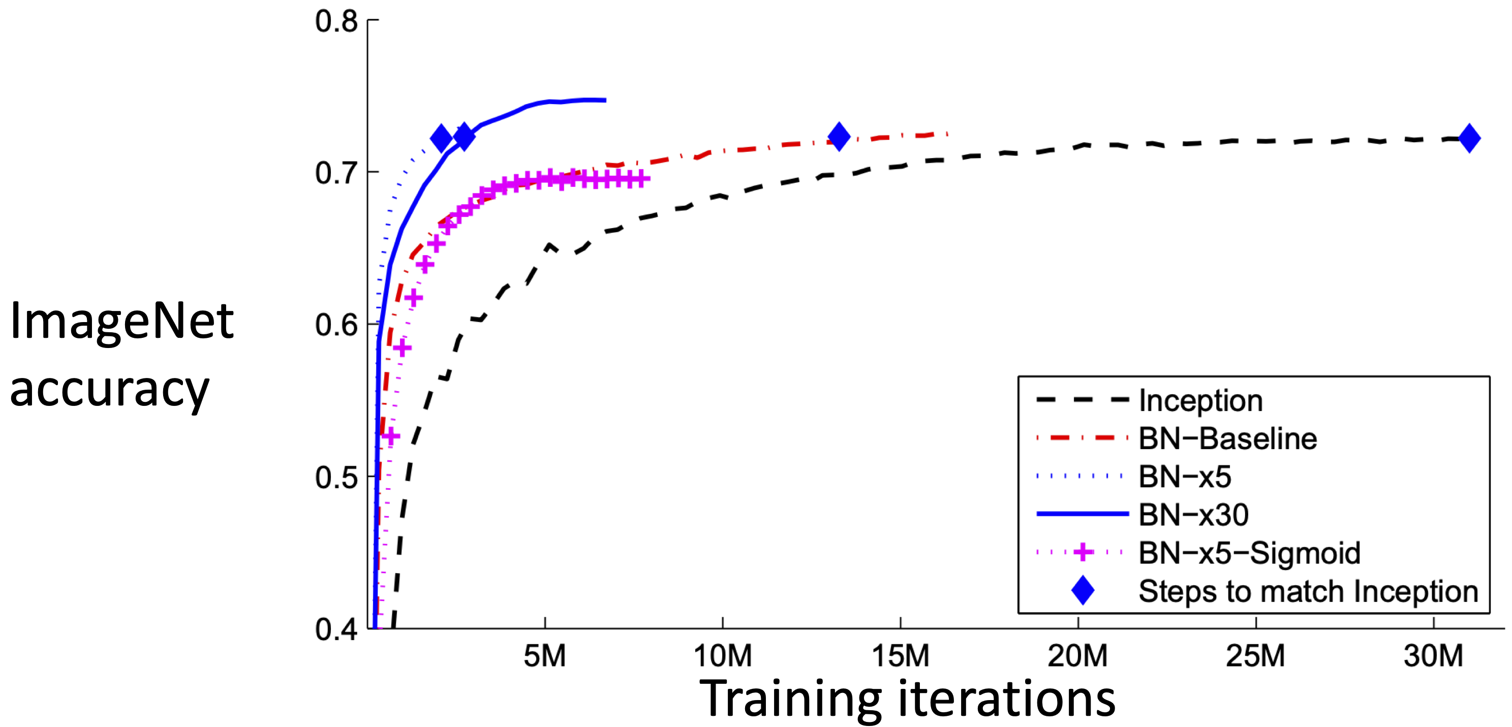
Does Batch Normalization Help?
- The Good:
- Makes deep networks much easier to train!
- Makes deep networks much easier to train!
- Allows higher learning rates, faster convergence
- Networks become more robust to initialization
- Acts as regularization during training
- Zero overhead at test-time: can be fused with conv!
- The Bad:
- Not well-understood theoretically (yet)
- Behaves differently during training and testing: this is a very common source of bugs!
Layer Normalization
Batch Normalization
$$\mathbf{x}: N\times D$$ Normalize $$ \begin{eqnarray} \mathbf{\mu},\mathbf{\sigma} &:& 1\times D \\ \mathbf{\gamma},\mathbf{\beta} &:& 1\times D\\ \mathbf{y} &=& \mathbf{\gamma}\frac{\mathbf{x}-\mathbf{\mu}}{\mathbf{\sigma}} + \mathbf{\beta} \end{eqnarray} $$
Layer Normalization
$$\mathbf{x}: N\times D$$ Normalize $$ \begin{eqnarray} \mathbf{\mu},\mathbf{\sigma} &:& N\times 1 \\ \mathbf{\gamma},\mathbf{\beta} &:& 1\times D \\ \mathbf{y} &=& \mathbf{\gamma}\frac{\mathbf{x}-\mathbf{\mu}}{\mathbf{\sigma}} + \mathbf{\beta} \end{eqnarray} $$
- Ba, Kiros, and Hinton, “Layer Normalization”, arXiv 2016
Instance Normalization
Batch Normalization
$$\mathbf{x}: N\times C\times H \times W$$ Normalize $$ \begin{eqnarray} \mathbf{\mu},\mathbf{\sigma} &:& 1\times C\times 1\times 1 \\ \mathbf{\gamma},\mathbf{\beta} &:& 1\times C\times 1\times 1 \\ \mathbf{y} &=& \mathbf{\gamma}\frac{\mathbf{x}-\mathbf{\mu}}{\mathbf{\sigma}} + \mathbf{\beta} \end{eqnarray} $$
Instance Normalization
$$\mathbf{x}: N\times C\times H \times W$$ Normalize $$ \begin{eqnarray} \mathbf{\mu},\mathbf{\sigma} &:& N\times C\times 1\times 1 \\ \mathbf{\gamma},\mathbf{\beta} &:& 1\times C\times 1\times 1 \\ \mathbf{y} &=& \mathbf{\gamma}\frac{\mathbf{x}-\mathbf{\mu}}{\mathbf{\sigma}} + \mathbf{\beta} \end{eqnarray} $$
- Ulyanov et al, Improved Texture Networks: Maximizing Quality and Diversity in Feed-forward Stylization and Texture Synthesis, CVPR 2017
Types of Normalization Layers
