Score Matching and Diffusion Models
CSE 891: Deep Learning
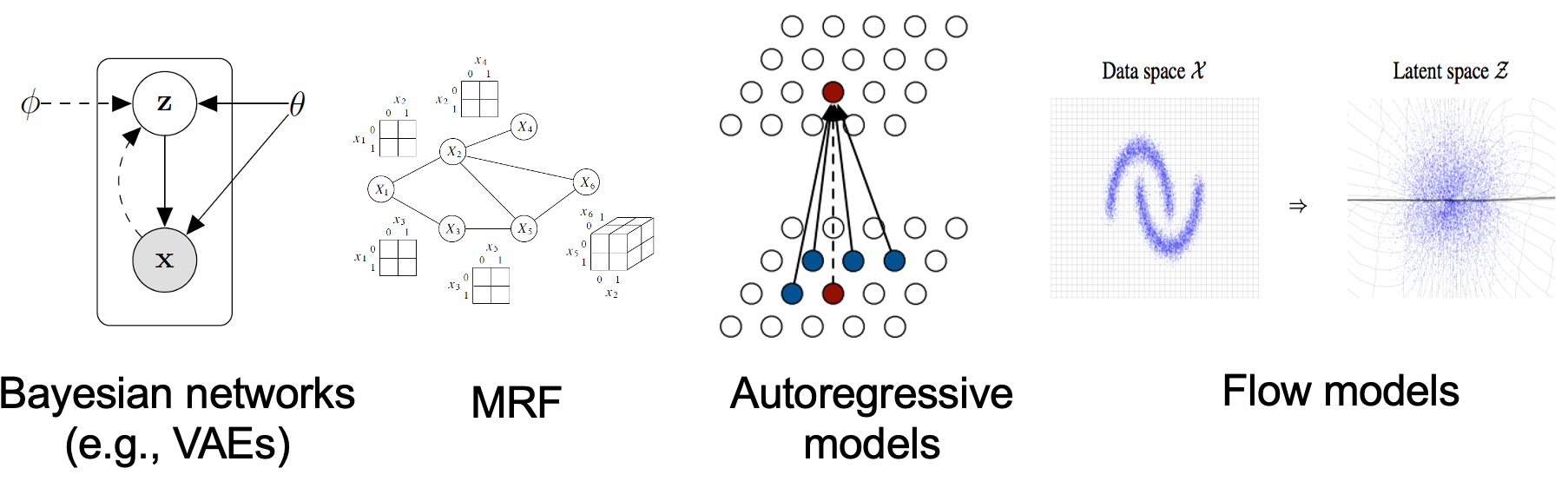
A Probabilistic Viewpoint
- Goal: modeling $p_{data}$


Likelihood vs Implicit

Maximum Likelihood
- Let $\{\mathbf{x}_1,\dots,\mathbf{x}_N\}$ be samples from an unknown distribution $p(\mathbf{x})$.
- Let $f_{\mathbf{\theta}}(\mathbf{x}) \in \mathbb{R}$ be a real-valued function with parameters $\mathbf{\theta}$. $$ p_{\mathbf{\theta}}(\mathbf{x}) = \frac{e^{-f_{\mathbf{\theta}}(\mathbf{x})}}{Z_{\mathbf{\theta}}} $$ where $Z_{\mathbf{\theta}}$ is a normalizing constant that depends on $\mathbf{\theta}$ such that $\int p_{\mathbf{\theta}}(\mathbf{x})d\mathbf{x} = 1$.
- Train $p_{\mathbf{\theta}}(\mathbf{x})$ through maximum log-likelihood of the data $$ \max_{\mathbf{\theta}}\sum_{i=1}^N \log p_{\mathbf{\theta}}(\mathbf{x}_i) = -f_{\mathbf{\theta}}(\mathbf{x}) - \log Z_{\mathbf{\theta}} $$
- Evaluating the normalizing constant $Z_{\mathbf{\theta}}$ is typically intractable for any general $f_{\mathbf{\theta}}(\mathbf{x})$.
Score Function
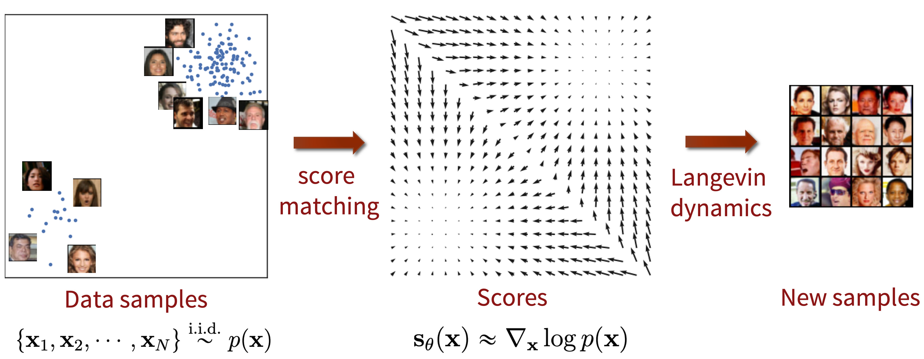
- Score function of $p(\mathbf{x})$ is defined as, $$ \nabla_{\mathbf{x}} \log p(\mathbf{x}) $$
- Learn a score based model $s_{\mathbf{\theta}}(\mathbf{x}) \approx \nabla_{\mathbf{x}} \log p(\mathbf{x})$

- Don't need to worry about normalizing constant. $$ s_{\mathbf{\theta}}(\mathbf{x}) \approx \nabla_{\mathbf{x}} \log p(\mathbf{x}) = -\nabla_{\mathbf{x}}f_{\mathbf{\theta}}(\mathbf{x}) - \underbrace{\nabla_{\mathbf{x}}\log Z_{\mathbf{\theta}}}_{0} = -\nabla_{\mathbf{x}}f_{\mathbf{\theta}}(\mathbf{x}) $$


- Image Credit: Yang Song
Learning: Score Matching
- Minimize Fischer Divergence between the model and the data distributions. $$ \max_{\mathbf{\theta}} \mathbb{E}_{p(\mathbf{x})}\left[\|\nabla_{\mathbf{x}}\log p(\mathbf{x}) - s_{\mathbf{\theta}}(\mathbf{x})\|_2^2\right] $$
- Problem: need access to unknown score of data i.e., $\nabla_{\mathbf{x}}\log p(\mathbf{x})$.
- Solution: Score matching algorithms minimize Fischer divergence without ground-truth data score. $$ \mathbb{E}_{p_{data}}\left[tr(\nabla^2_{\mathbf{x}}\log p_{\mathbf{\theta}}(\mathbf{x}) + \frac{1}{2}\|\nabla_{\mathbf{x}}\log p_{\mathbf{\theta}}(\mathbf{x})\|_2^2\right] $$
- Practical realizations:
- Sliced Score Matching (Yang 2019): $\mathbb{E}_{p_{data}}\left[\mathbf{v}^T\nabla^2_{\mathbf{x}}\log p_{\mathbf{\theta}}(\mathbf{x})\mathbf{v} + \frac{1}{2}(\mathbf{v}^T\nabla_{\mathbf{x}}\log p_{\mathbf{\theta}}(\mathbf{x})\mathbf{v})^2\right]$
- Denoising Autoencoders (Vincent 2011): $\mathbb{E}_{p_{data}(\mathbf{x})}\mathbb{E}_{\tilde{\mathbf{x}} \sim \mathcal{N}(\mathbf{x},\sigma^2\mathbf{I})}\left[\|s_{\mathbf{\theta}}(\tilde{\mathbf{x}, \sigma}) + \frac{\tilde{\mathbf{x}}-\mathbf{x}}{\sigma^2}\|_2^2\right]$
Sampling: Langevin Dynamics
- Score function, $s_{\mathbf{\theta}}(\mathbf{x}) \approx \nabla_{\mathbf{x}}p(\mathbf{x})$, can be used to draw samples from it through an iterative procedure called Langevin Dynamics.
- Langevin dynamics provides an MCMC procedure to sample from a $p(\mathbf{x})$ using only its score function $\nabla_{\mathbf{x}}p(\mathbf{x})$. $$\mathbf{x}_0 \sim \pi(\mathbf{x})$$ $$\mathbf{x}_{i+1} \leftarrow \mathbf{x}_i + \epsilon\nabla_{\mathbf{x}}\log p(\mathbf{x}) + \sqrt{2\epsilon}\mathbf{z}_i, i=0,1,\dots,K$$
- Langevin dynamics accesses $p(\mathbf{x})$ only through $\nabla_{\mathbf{x}}p(\mathbf{x})$.
- Since $s_{\mathbf{\theta}}(\mathbf{x}) \approx \nabla_{\mathbf{x}}p(\mathbf{x})$, we can produce samples from $s_{\mathbf{\theta}}(\mathbf{x})$.
Summary: Score-Based Generative Models
Pitfalls of Naive Score-Based Models
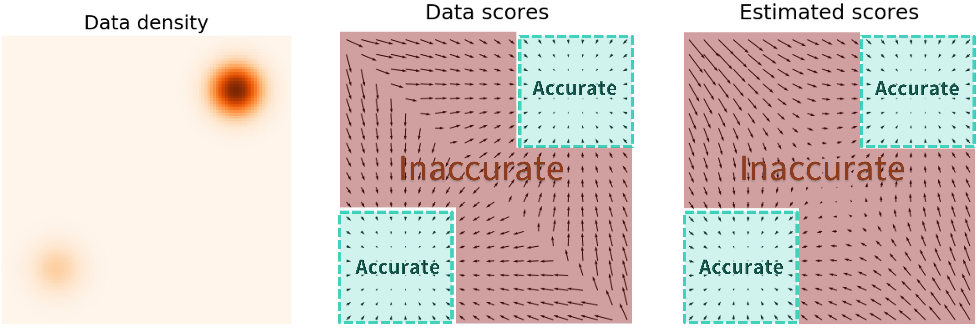
- Inaccurate score predictions will derail Langevin dynamics and lead to poor quality generated samples.
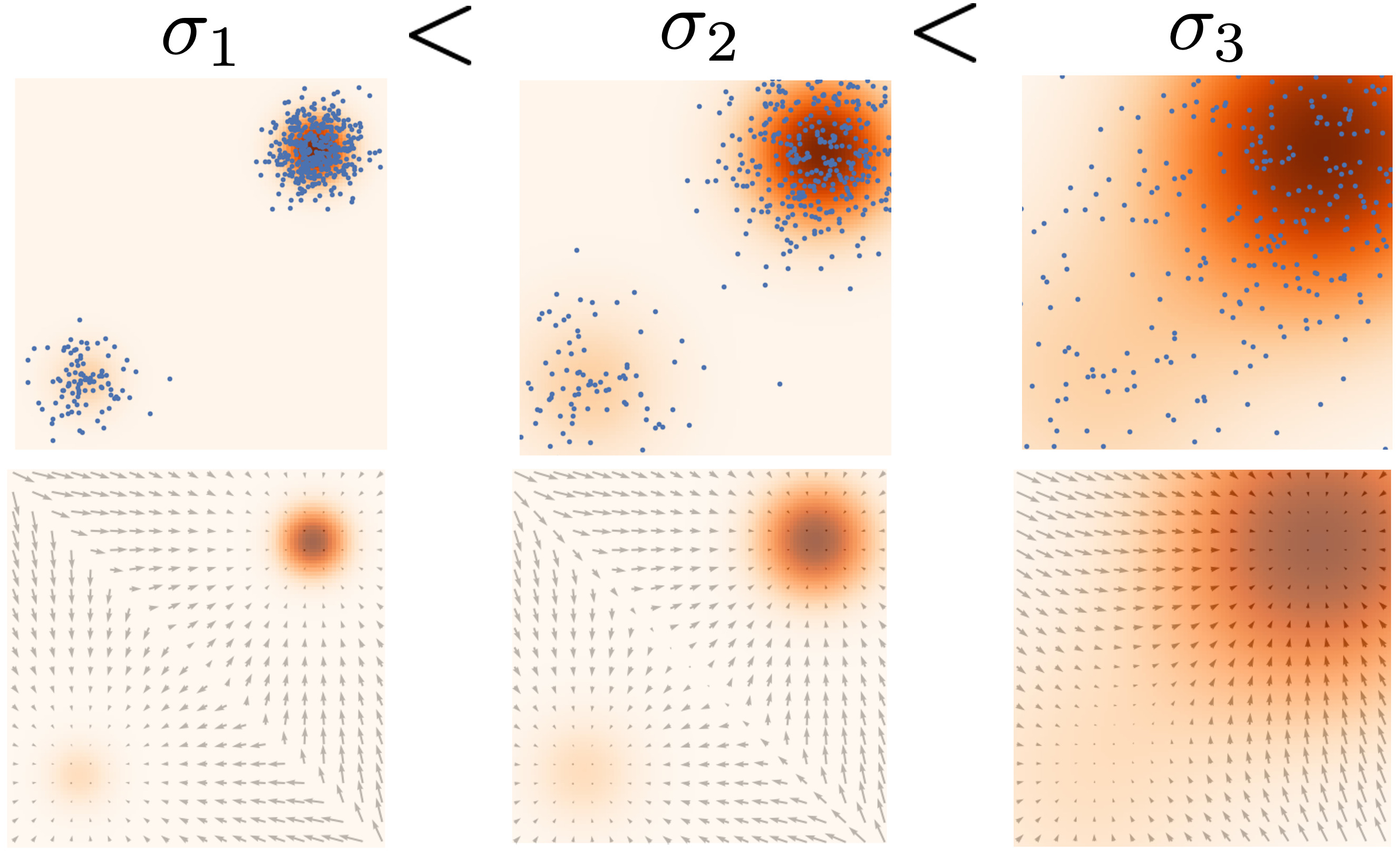
Generative Modeling with Multiple Noise Perturbations
- Problem: How to overcome difficulty of score estimation in low-density regions?
- Solution: Train score-based models on perturbations of data.
- Perturbation with noise is equivalent to convolution.
- $z = x + y \Longrightarrow p(z) = p(x) \ast p(y)$

- How do we choose the appropriate noise scale?
- Image Credit: Yang Song
Generative Modeling with Multiple Noise Perturbations
- Larger noise covers more low density regions, but it alters the original distribution significantly.
- Smaller noise does not alter the original distribution, but it does not cover low density regions.
- Solution: Use multiple scales of noise perturbations simultaneously.
- For $L$ increasing standard deviations $\sigma_1 < \sigma_2 < \cdots < \sigma_L$, perturb data with Gaussian noise $\mathcal{N}(\mathbf{0}, \sigma_i^2\mathbf{I})$ i.e., $$ p_{\sigma_i}(\mathbf{x}) = \int p(\mathbf{y})\mathcal{N}(\mathbf{x};\mathbf{y},\sigma_i^2\mathbf{I})d\mathbf{y} $$
- Noise Conditional Score-Based Model: $\mathbf{s}_{\mathbf{\theta}}(\mathbf{x},i) \approx \nabla_{\mathbf{x}}\log p_{\sigma_i}(\mathbf{x})$
Generative Modeling with Multiple Noise Perturbations
Noise Conditional Score-Based Model
$$ \sum_{i=1}^L \lambda(i)\mathbb{E}_{p_{\sigma_i}(\mathbf{x})}\left[\|\nabla_{\mathbf{x}}\log p_{\sigma_i}(\mathbf{x}) - \mathbf{s}_{\mathbf{\theta}}(\mathbf{x},i)\|_2^2\right] $$- where $\lambda(i) \in \mathbb{R}_{> 0}$, and typically $\lambda(i) = \sigma_i^2$.
- Sample from $\mathbf{s}_{\mathbf{\theta}}(\mathbf{x},i)$ from $i=L, L-1, \dots, 1$

Noise Conditional Score-Based Model
- Practical implementation design choices:
- Choose $\sigma_1 < \sigma_2 < \cdots < \sigma_L$ as a geometric progression, $L \sim 1000s$
- $\mathbf{s}_{\mathbf{\theta}}(\mathbf{x},i)$ is modeled by a U-Net architecture with skip-connections.
- Apply EMA on the weights of the score-based model when used at test-time.

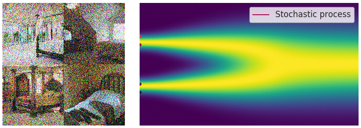
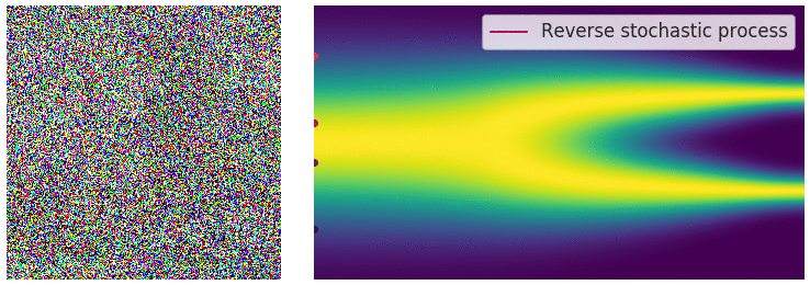
Perturbing Data with Stochastic Differential Equations
- When $L \rightarrow \infty$, we perturb the data with continuously growing levels of noise.
- Stochastic processes are typically solutions of stochastic differential equations (SDEs). $$ d\mathbf{x} = f(\mathbf{x},t)dt + g(t)d\mathbf{w} $$
- $f(\cdot,t):\mathbb{R}^d \rightarrow \mathbb{R}^d$ is a vector-valued function called the drift coefficient.
- $g(t) \in \mathbb{R}$ is a real-valued function called the diffusion coefficient
- $\mathbf{w}$ is standard Brownian motion, and $d\mathbf{w}$ is infinitesimal white noise.
Sample Generation by Reversing Stochastic Differential Equation
- Any SDE has a corresponding reverse SDE. $$ d\mathbf{x} = [f(\mathbf{x},t) - g^2(t)\nabla_{\mathbf{x}}\log p_t(\mathbf{x})]dt + g(t)d\mathbf{w} $$
- $dt$ is a negative infinitesimal time step.
- $\nabla_{\mathbf{x}}\log p_t(\mathbf{x})$ is exactly the score function.
Summary: Stochastic Differential Equations

How does it perform?
| Method | FID($\downarrow$) | Inception Score($\uparrow$) |
|---|---|---|
| StyleGAN2 + ADA | 2.92 | 9.83 |
| Score-Based SDE | 2.20 | 9.89 |

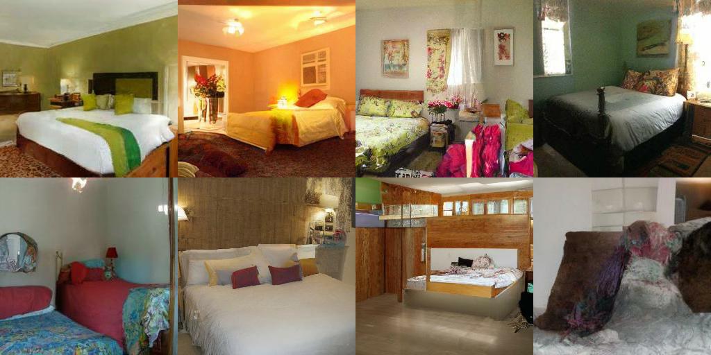
Examples Images

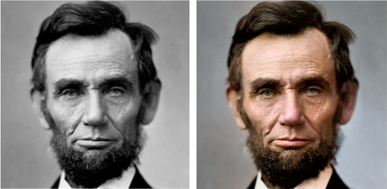
Controllable Generation for Solving Inverse Problems
- Inverse problems involve estimating a sample $\mathbf{x}$ given information $\mathbf{y}$
- Can be solved as, $p(x|y) = p(x)p(y|x)$, so, $$ \nabla_{\mathbf{x}}\log p(\mathbf{x}|\mathbf{y})=\nabla_{\mathbf{x}}\log p(\mathbf{x}) + \nabla_{\mathbf{x}}\log p(\mathbf{y}|\mathbf{x}) $$
- $p(y|x)$ is a classifier. All we need to turn an unconditional diffusion model into a conditional one, is a classifier !!
- An additional scaling factor is usually added to increase the temperature of $p(y|x)$. $$ \nabla_{\mathbf{x}}\log p(\mathbf{x}|\mathbf{y})=\nabla_{\mathbf{x}}\log p(\mathbf{x}) + \gamma\nabla_{\mathbf{x}}\log p(\mathbf{y}|\mathbf{x}) $$
Controllable Generation for Solving Inverse Problems
- Problem: Difficult to obtain noise-robust classifier.
- Solution: Classifier-free guidance. Observe that $p(y|x) = \frac{p(x|y)p(y)}{p(x)}$, so, $$ \begin{aligned} \nabla_{x}\log p(y|x) &= \nabla_{x}\log p(x|y) - \nabla_x \log p(x) \\ \nabla_{x}\log p_{\gamma}(x|y) &= \nabla_{x}\log p(x) +\gamma(\nabla_{x}\log p(x|y) - \nabla_x \log p(x)) \\ \nabla_{x}\log p_{\gamma}(x|y) &= (1-\gamma)\nabla_{x}\log p(x) + \gamma\nabla_{x}\log p(x|y) \end{aligned} $$
- This is a barycentric combination of the conditional and unconditional score function.
- When $\gamma=1$, we recover the conditional model.
- When $\gamma=0$, we recover the unconditional model.
Inverse Problem Examples
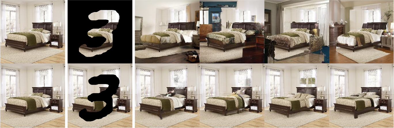

Inverse Problem Examples
Diffusion Models
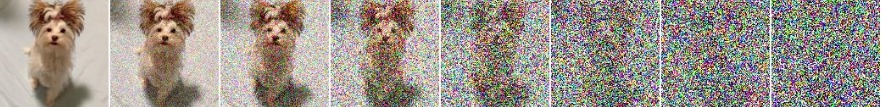
- Denoising diffusion models consist of two processes:
- Forward diffusion process:
- gradually adds noise to input
- the variance of the noise increases with iterations
- Reverse denoising process:
- learns to generate data by denoising

Diffusion Models: Forward Process
- Forward process is executed for $T$ steps:
 $$
\begin{aligned}
q(\mathbf{x}_t|\mathbf{x}_{t-1}) = \mathcal{N}(\mathbf{x}_t;\sqrt{1-\beta_t}\mathbf{x}_{t-1}, \beta_t\mathbf{I}) &\rightarrow q(\mathbf{x}_{1:T}|\mathbf{x}_0) = \prod_{t=1}^T q(\mathbf{x}_t|\mathbf{x}_{t-1}) \mbox{ (joint)} \\
\bar{\alpha}_t = \prod_{s=1}^t (1-\beta_s) \rightarrow q(\mathbf{x}_t|\mathbf{x}_0) &= \mathcal{N}(\mathbf{x}_t;\sqrt{\bar{\alpha}_t}\mathbf{x}_0, (1-\bar{\alpha}_t)\mathbf{I}) \mbox{ (Diffusion Kernel)} \\
\mbox{For sampling: } \mathbf{x}_t = \sqrt{\bar{\alpha}_t}\mathbf{x}_0 &+ \sqrt{1-\bar{\alpha}_t}\mathbf{\epsilon} \mbox{ where } \mathbf{\epsilon} \sim \mathcal{N}(\mathbf{0},\mathbf{I})
\end{aligned}
$$
$$
\begin{aligned}
q(\mathbf{x}_t|\mathbf{x}_{t-1}) = \mathcal{N}(\mathbf{x}_t;\sqrt{1-\beta_t}\mathbf{x}_{t-1}, \beta_t\mathbf{I}) &\rightarrow q(\mathbf{x}_{1:T}|\mathbf{x}_0) = \prod_{t=1}^T q(\mathbf{x}_t|\mathbf{x}_{t-1}) \mbox{ (joint)} \\
\bar{\alpha}_t = \prod_{s=1}^t (1-\beta_s) \rightarrow q(\mathbf{x}_t|\mathbf{x}_0) &= \mathcal{N}(\mathbf{x}_t;\sqrt{\bar{\alpha}_t}\mathbf{x}_0, (1-\bar{\alpha}_t)\mathbf{I}) \mbox{ (Diffusion Kernel)} \\
\mbox{For sampling: } \mathbf{x}_t = \sqrt{\bar{\alpha}_t}\mathbf{x}_0 &+ \sqrt{1-\bar{\alpha}_t}\mathbf{\epsilon} \mbox{ where } \mathbf{\epsilon} \sim \mathcal{N}(\mathbf{0},\mathbf{I})
\end{aligned}
$$
Diffusion Models: Reverse Denoising Process
- Reverse process is executed for $T$ steps:
 $$
\begin{aligned}
p(\mathbf{x}_T) = \mathcal{N}(\mathbf{x}_T;\mathbf{0},\mathbf{I}) \mbox{ and } &p_{\mathbf{\theta}}(\mathbf{x}_{t-1}|\mathbf{x}_t) = \mathcal{N}(\mathbf{x}_{t-1};\mathbf{\mu}_{\mathbf{\theta}}(\mathbf{x}_t,t), \sigma_t^2\mathbf{I}) \\
p_{\mathbf{\theta}}(\mathbf{x}_{0:T}) &= p(\mathbf{x}_T)\prod_{t=1}^Tp_{\mathbf{\theta}}(\mathbf{x}_{t-1}|\mathbf{x}_t)
\end{aligned}
$$
$$
\begin{aligned}
p(\mathbf{x}_T) = \mathcal{N}(\mathbf{x}_T;\mathbf{0},\mathbf{I}) \mbox{ and } &p_{\mathbf{\theta}}(\mathbf{x}_{t-1}|\mathbf{x}_t) = \mathcal{N}(\mathbf{x}_{t-1};\mathbf{\mu}_{\mathbf{\theta}}(\mathbf{x}_t,t), \sigma_t^2\mathbf{I}) \\
p_{\mathbf{\theta}}(\mathbf{x}_{0:T}) &= p(\mathbf{x}_T)\prod_{t=1}^Tp_{\mathbf{\theta}}(\mathbf{x}_{t-1}|\mathbf{x}_t)
\end{aligned}
$$
- $\mathbf{\mu}_{\mathbf{\theta}}(\mathbf{x}_t,t) \mbox{: Trainable Network (U-Net, Denoising Autoencoder)}$
- Conceptually, the network learns to predict and subtract the noise that was added in the forward pass.
Connection to Diffusion Models
- Diffusion models and score-based models are different perspectives of the same underlying class of generative models.
- Both perturb data with multiple scales of noise.
- The loss function for training diffusion models is equivalent to the weighted combination of score matching objectives.
State-of-the-Art
- OpenAI DALL$\cdot$E 2 (see next few slides)
- Google Imagen (see next few slides)