Constraint Satisfaction - II
CSE 440: Introduction to Artificial Intelligence
Content Credits: CMU AI, http://ai.berkeley.edu
Today
- Solving CSPs: Backtracking Search
- Filtering
- Ordering
- Problem Structure

- Reading
- Today's Lecture: RN Chapter 6
- Next Lecture: RN Chapter 5.1-5.3
Backtracking Search
Backtracking Search
- Backtracking search is the basic uninformed algorithm for solving CSPs
- Idea 1: One variable at a time
- Variable assignments are commutative, so fix ordering
- Problem is commutative if order of application of any given set of actions has no effect on outcome.
- i.e., [WA = red then NT = green] same as [NT = green then WA = red]
- Only need to consider assignments to a single variable at each step
- Idea 2: Check constraints as you go
- i.e. consider only values which do not conflict with previous assignments
- Might have to do some computation to check the constraints
- "Incremental goal test"
- DFS with these two improvements is called backtracking search (not the best name)
- Can solve n-queens for $n \approx 25$
Backtracking Example


Backtracking Search
Improving Backtracking Search
- General-purpose ideas give huge gains in speed
- Backtracking is an uninformed algorithm. So we don't expect it to be very effective for large problems. We know the informed search can improve the efficiency and effectiveness.
- Ordering:
- Which variable should be assigned next?
- In what order should its values be tried?
- Filtering: Can we detect inevitable failure early?
- Structure: Can we exploit the problem structure?
Ordering
Ordering: Minimum Remaining Values
- Variable Ordering: Minimum remaining values (MRV):
- Choose the variable with the fewest legal values left in its domain
- Why min rather than max?
- Also called "most constrained variable"
- "Fail-fast" ordering


Ordering: Least Constraining Value
- Value Ordering: Least Constraining Value
- Given a choice of variable, choose the least constraining value
- i.e., the one that rules out the fewest values in the remaining variables
- Why least rather than most?
- Combining these ordering ideas makes 1000 queens feasible
Filtering
Filtering: Forward Checking
- Filtering: Keep track of domains for unassigned variables and cross off bad options.
- Forward checking: Cross off values that violate a constraint when added to the existing assignment


Filtering: Constraint Propagation
- Forward checking propagates information from assigned to unassigned variables, but doesn't provide early detection for all failures:
- NT and SA cannot both be blue!
- Why didn’t we detect this yet?
- Constraint propagation: reason from constraint to constraint
Consistency of A Single Arc
- An arc $X \rightarrow Y$ is consistent iff for every $x$ in the tail there is some $y$ in the head which could be assigned without violating a constraint.


- Forward checking: Enforcing consistency of arcs pointing to each new assignment.
- Delete from the tail !!
Arc Consistency of an Entire CSP
- A simple form of propagation makes sure all arcs are consistent:

- Important: If X loses a value, neighbors of X need to be rechecked.
- Arc consistency detects failure earlier than forward checking
- Can be run as a preprocessor or after each assignment
- What is the downside of enforcing arc consistency?
Enforcing Arc Consistency in a CSP
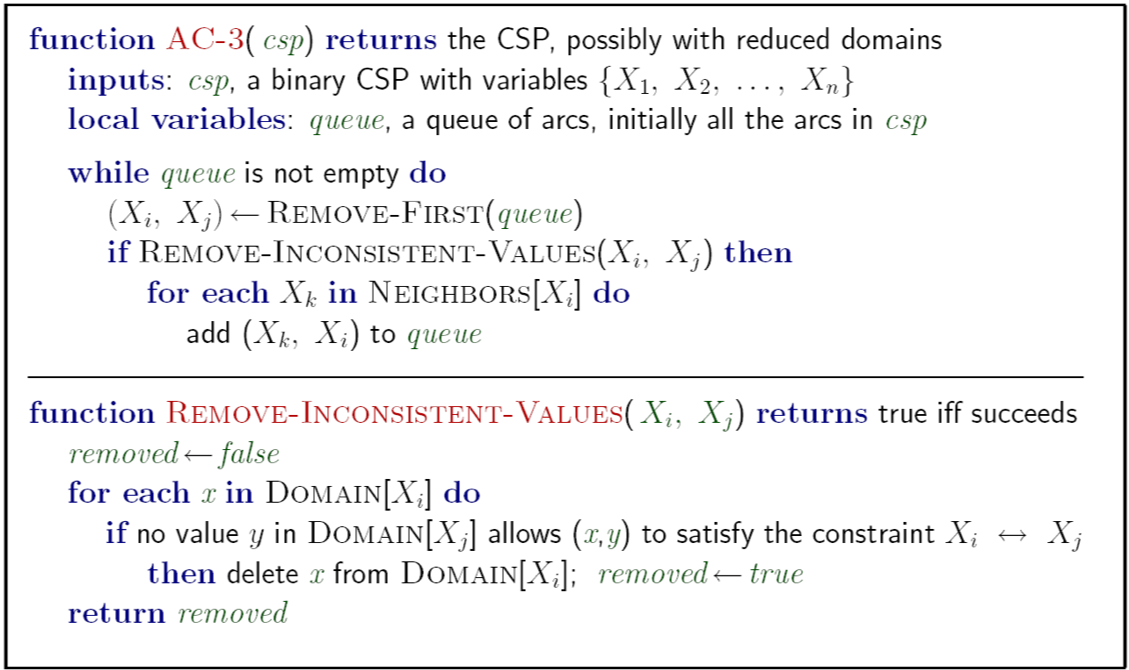
- Runtime: $\mathcal{O}(n^2d^3)$, can be reduced to $\mathcal{O}(n^2d^2)$
- But detecting all possible future problems is NP-hard.
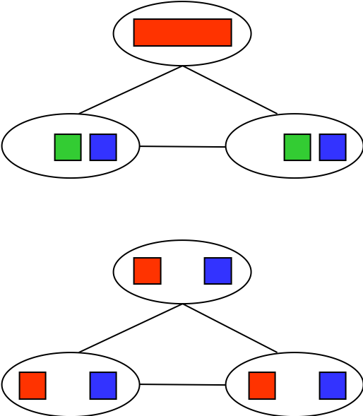
Limitations of Arc Consistency
- After enforcing arc consistency:
- Can have one solution left
- Can have multiple solutions left
- Can have no solutions left (and not know it)
- Arc consistency still runs inside a backtracking search.
Problem Structure
Problem Structure
- Real world problem can be decomposed into many subproblems.
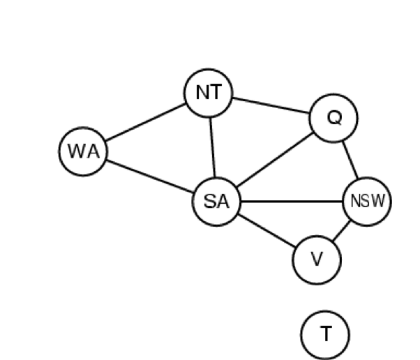
- Extreme case: independent subproblems
- Tasmania and mainland are independent subproblems
- Independent subproblems are identifiable as connected components of constraint graph
- Suppose a graph of $n$ variables can be broken into subproblems of only $c$ variables:
- Worst-case solution cost is $\mathcal{O}((n/c)(d^c))$, linear in $n$
- E.g., $n = 80$, $d = 2$, $c =20$
- $2^{80} = 4$ billion years at 10 million nodes/sec
- $(4)(2^{20}) = 0.4$ seconds at 10 million nodes/sec
Problem Structure
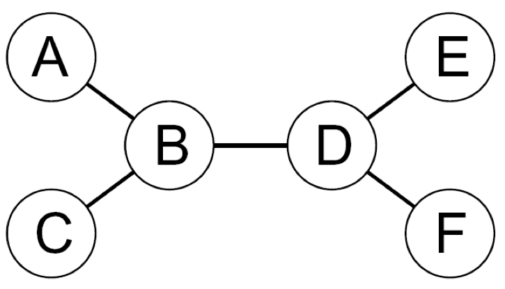
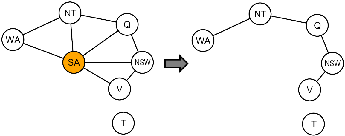
- Theorem: if the constraint graph has no loops, the CSP can be solved in $\mathcal{O}(nd^2)$ time
- Compare to general CSPs, where worst-case time is $\mathcal{O}(d^n)$
- This property also applies to probabilistic reasoning (later): an example of the relation between syntactic restrictions and the complexity of reasoning.
Problem Structure
- Algorithm for tree-structured CSPs:
- Order: Choose a root variable, order variables so that parents precede children
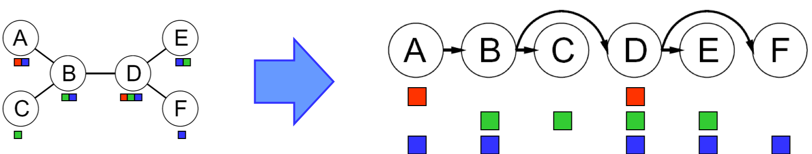
- Remove backward: For $i = n : 2$, apply RemoveInconsistent(Parent($X_i$),$X_i$)
- Assign forward: For $i = 1 : n$, assign $X_i$ consistently with Parent($X_i$)
- Runtime: $\mathcal{O}(nd^2)$
Problem Structure
- Conditioning: instantiate a variable, prune its neighbors' domains
- Cutset conditioning: instantiate (in all ways) a set of variables such that the remaining constraint graph is a tree
- Cutset size $c$ gives runtime $\mathcal{O}((d^c)(n-c)d^2)$, very fast for small $c$.
Q & A