Reinforcement Learning - III
CSE 440: Introduction to Artificial Intelligence
Content Credits: CMU AI, http://ai.berkeley.edu
Today
- Approximate $Q$-Learning
- Applications of RL
Reinforcement Learning
- Still assume a Markov decision process (MDP):
- A set of states $s \in S$
- A set of states per state $A$
- A model $T(s,a,s')$
- A reward function $R(s,a,s')$
- Still looking for a policy $\pi(s)$
- New twist: do not know $T$ or $R$
- Big idea: Compute all averages over $T$ using sample outcomes
Recap: $Q$-Learning
- $Q$-Learning: sample-based $Q$-value iteration $$\begin{equation} Q_{k+1}(s,a) \leftarrow \sum_{s'}T(s,a,s')[R(s,a,s') + \gamma \max_{a'}Q_k(s',a')] \end{equation}$$
- Learn $Q(s,a)$ values as you go
- Receive a sample $(s,a,s',r)$
- Consider your old estimate: $Q(s,a)$
- Consider your new sample estimate: $$\begin{equation} sample = R(s,a,s') + \gamma \max_{a'}Q(s',a') \end{equation}$$
- Incorporate the new estimate into a running average: $$\begin{equation} Q(s,a) \leftarrow (1-\alpha)Q(s,a) + (\alpha) sample \end{equation}$$
Approximate $Q$-Learning
Generalizing Across States
- Basic $Q$-Learning keeps a table of all q-values
- In realistic situations, we cannot possibly learn about every single state.
- Too many states to visit them all in training
- Too many states to hold the q-tables in memory
- Instead, we want to generalize:
- Learn about some small number of training states from experience
- Generalize that experience to new, similar situations
- This is a fundamental idea in machine learning, and we will see it over and over again
Example: Pacman
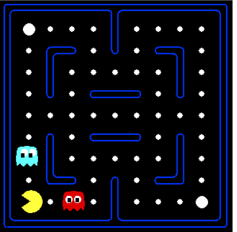


Feature-Based Representations
- Solution: describe a state using a vector of features (properties)
- Features are functions from states to real numbers (often 0/1) that capture important properties of the state
- Example features:
- Distance to closest ghost
- Distance to closest dot
- Number of ghosts
- $\frac{1}{(\mbox{dist to dots})^2}$
- Is Pacman in a tunnel? (0/1)
- $\dots$ etc.
- Is it the exact state on this slide?
- Can also describe a $q$-state (s, a) with features (e.g. action moves closer to food)
Linear Value Functions
- Using a feature representation, we can write a $q$ function (or value function) for any state using a few weights: $$\begin{equation} \begin{aligned} V(s) = w_1f_1(s) + w_2f_2(s) + \dots + w_nf_n(s) \nonumber \\ Q(s,a) = w_1f_1(s,a) + w_2f_2(s,a) + \dots + w_nf_n(s,a) \nonumber \\ \end{aligned} \end{equation}$$
- Advantage: our experience is summed up in a few powerful numbers
- Disadvantage: states may share features but actually be very different in value.
Approximate $Q$-Learning
$Q(s,a) = w_1f_1(s,a) + w_2f_2(s,a) + \dots + w_nf_n(s,a)$
- Q-learning with linear Q-functions: $$\begin{equation} transition = (s,a,r,s') \end{equation}$$ $$\begin{equation} difference = [r + \gamma \max_{a'}Q(s',a')] - Q(s,a) \end{equation}$$ $$\begin{equation} Q(s,a) \leftarrow Q(s,a) + \alpha[difference] \mbox{ Exact Q's} \end{equation}$$ $$\begin{equation} w_i \leftarrow w_i + \alpha[difference]f_i(s,a) \mbox{ Approximate Q's} \end{equation}$$
- Intuitive interpretation:
- Adjust weights of active features
- E.g., if something unexpectedly bad happens, blame the features that were on: do not prefer all states with that state's features
- Formal justification: online least squares
Example $Q$-Pacman


$Q$-Learning and Least Squares
Linear Approximation: Regression

Optimization: Least Squares
$$\begin{equation} \mbox{total error } = \sum_i (y_i-\hat{y}_i)^2 = \sum_i \left(y_i - \sum_k w_kf_k(x)\right)^2 \end{equation}$$
Minimizing Error
- Imagine we had only one point x, with features f(x), target value y, and weights w:
-
$$\begin{equation}
error(w) = \frac{1}{2}\left(y-\sum_k w_kfk(x)\right)^2
\end{equation}$$
$$\begin{equation}
\frac{\partial error(w)}{\partial w_m} = -\left(y-\sum_k w_kfk(x)\right)f_m(x)
\end{equation}$$
$$\begin{equation}
w_m \leftarrow w_m + \alpha\left(y-\sum_k w_kfk(x)\right)f_m(x)
\end{equation}$$
- Approximate q update explained: $$\begin{equation} w_m \leftarrow w_m + \alpha[\underbrace{r + \gamma\max_{a}Q(s',a')}_{"target"}-\underbrace{Q(s,a)}_{"prediction"}]f_m(s,a) \nonumber \end{equation}$$
Applications
RL: Helicopter Flight
RL: Learning Locomotion
RL: Learning Soccer
RL: Learning Manipulation
RL: NASA SUPERBall
RL: In-Hand Manipulation
Conclusion
- We are done with Part I: Search and Planning
- We have seen how AI methods can solve problems in:
- Search
- Constraint Satisfaction Problems
- Optimization
- Markov Decision Problems
- Reinforcement Learning
- Next Up: Part II: Uncertainty
Q & A