Probability
CSE 440: Introduction to Artificial Intelligence
Vishnu Boddeti
Content Credits: CMU AI, http://ai.berkeley.edu
Today
- Random Variables
- Joint and Marginal Probabilities
- Conditional Probabilities
- Product Rule, Chain Rule, Bayes Rule
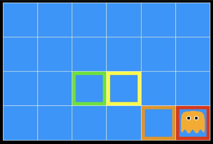
Inference in Ghostbusters
- A ghost is in the grid somewhere
- Sensor readings tell how close a square is to the ghost
- On the ghost: red
- 1 or 2 away: orange
- 3 or 4 away: yellow
- 5+ away: green
Sensors are noisy, but we know $P(color|distance)$
| $pred(red|3)$ |
$pred(orange|3)$ |
$pred(yellow|3)$ |
$pred(green|3)$ |
| 0.05 |
0.15 |
0.50 |
0.30 |
Uncertainty
- General situation:
- Observed variables (evidence): Agent knows certain things about the state of the world (e.g., sensor readings or symptoms)
- Unobserved variables: Agent needs to reason about other aspects (e.g. where an object is or what disease is present)
- Model: Agent knows something about how the known variables relate to the unknown variables
- Probabilistic reasoning gives us a framework for managing our beliefs and knowledge
| 0.11 |
0.11 |
0.11 |
| 0.11 |
0.11 |
0.11 |
| 0.11 |
0.11 |
0.11 |
| 0.17 |
0.10 |
0.10 |
| 0.09 |
0.17 |
0.10 |
| 0.01 |
0.09 |
0.17 |
| 0.01 |
0.01 |
0.03 |
| 0.01 |
0.05 |
0.05 |
| 0.01 |
0.05 |
0.81 |
Random Variables
- A random variable is some aspect of the world about which we (may) have uncertainty
- $R =$ Is it raining?
- $T =$ Is it hot or cold?
- $D =$ How long will it take to drive to work?
- $L =$ Where is the ghost?
- We denote random variables with capital letters
- Like variables in a CSP, random variables have domains
- $R \in \{false, true\}$ (often written as $\{-r, +r\}$)
- $T \in \{hot, cold\}$
- $D \in [0, \infty)$
- $L \in \mbox{ possible locations}$, maybe $\{(0,0), (0,1), \dots\}$
Probability Distributions
- Associate a probability with each value
Weather $P(W)$
| $W$ |
$P$ |
| sun |
0.6 |
| rain |
0.1 |
| fog |
0.3 |
| meteor |
0.0 |
Probability Distributions
- Unobserved random variables have distributions
- A distribution is a TABLE of probabilities of values
- A probability (lower case value) is a single number $P(W=rain)=0.1$
- Must have: \[\forall x \mbox{ } P(X=x) \geq 0\] and \[\sum_x P(X=x)=1\]
Shorthand Notation:
\begin{equation}
\begin{aligned}
P(hot) &= P(T=hot) \nonumber \\
P(cold) &= P(T=cold) \nonumber \\
P(rain) &= P(W=rain) \nonumber \\
\end{aligned}
\end{equation}
OK, if all domains entries are unique
Joint Distributions
- A joint distribution over a set of random variables: $X_1,X_2,\dots,X_n$
- Joint distribution specifies a real number for each assignment (or outcome):
\begin{equation}
\begin{aligned}
& P(X_1,\dots,X_n)\nonumber \\
& P(X_1=x_1,\dots,X_n=x_n)\nonumber
\end{aligned}
\end{equation}
- Must obey:
\begin{equation}
\begin{aligned}
& P(x_1,x_2,\dots,x_n) \geq 0 \nonumber \\
& \sum_{x_1,\dots,x_n} P(x_1,x_2,\dots,x_n) = 1 \nonumber
\end{aligned}
\end{equation}
- Size of distribution if n variables with domain sizes d?
- For all but the smallest distributions, impractical to write out !!
| $T$ |
$W$ |
$P$ |
| hot |
sun |
0.4 |
| hot |
rain |
0.1 |
| cold |
sun |
0.2 |
| cold |
rain |
0.3 |
Probabilistic Models
- A probabilistic model is a joint distribution over a set of random variables
- Probabilistic models:
- (Random) variables with domains
- Assignments are called outcomes
- Joint distributions: say whether assignments (outcomes) are likely
- Normalized: sum to 1.0
- Ideally: only certain variables directly interact
- Constraint satisfaction problems:
- Variables with domains
- Constraints: state whether assignments are possible
- Ideally: only certain variables directly interact
| $T$ |
$W$ |
$P$ |
| hot |
sun |
0.4 |
| hot |
rain |
0.1 |
| cold |
sun |
0.2 |
| cold |
rain |
0.3 |
| $T$ |
$W$ |
$P$ |
| hot |
sun |
T |
| hot |
rain |
F |
| cold |
sun |
F |
| cold |
rain |
T |
Events
- An event is a set E of outcomes:
\begin{equation}
P(E) = \sum_{(x_1,\dots,x_n)\in E} P(x_1,\dots,x_n) \nonumber
\end{equation}
- From a joint distribution, we can calculate the probability of any event
- Probability that it is hot AND sunny?
- Probability that it is hot?
- Probability that it is hot OR sunny?
- Typically, the events we care about are partial assignments, like $P(T=hot)$
| $T$ |
$W$ |
$P$ |
| hot |
sun |
0.4 |
| hot |
rain |
0.1 |
| cold |
sun |
0.2 |
| cold |
rain |
0.3 |
Marginal Distributions
- Marginal distributions are sub-tables which eliminate variables
- Marginalization (summing out): Combine collapsed rows by adding
| $T$ |
$W$ |
$P$ |
| hot |
sun |
0.4 |
| hot |
rain |
0.1 |
| cold |
sun |
0.2 |
| cold |
rain |
0.3 |
Conditional Distributions
- A simple relation between joint and conditional probabilities
- In fact, this is taken as the definition of a conditional probability
\begin{equation}
P(a|b) = \frac{P(a,b)}{P(b)} \nonumber
\end{equation}
| $T$ |
$W$ |
$P$ |
| hot |
sun |
0.4 |
| hot |
rain |
0.1 |
| cold |
sun |
0.2 |
| cold |
rain |
0.3 |
\begin{equation}
P(W=s|T=c) = \frac{P(W=s,T=c)}{P(T=c)} = \frac{P(W=s,T=c)}{P(W=s,T=c)+P(W=r,T=c)} = \frac{0.2}{0.2+0.3} = 0.4 \nonumber
\end{equation}
Conditional Distributions
- Conditional distributions are probability distributions over some variables given fixed values of others
$P(W|T=hot)$
$P(W|T=cold)$
| $T$ |
$W$ |
$P$ |
| hot |
sun |
0.4 |
| hot |
rain |
0.1 |
| cold |
sun |
0.2 |
| cold |
rain |
0.3 |
Normalization Tricks
| $T$ |
$W$ |
$P$ |
| hot |
sun |
0.4 |
| hot |
rain |
0.1 |
| cold |
sun |
0.2 |
| cold |
rain |
0.3 |
Normalization Tricks
- Why does this work?
- Sum of selection is P(evidence)!
- $P(T=c)$ in this case
- In general:
\begin{equation}
P(x_1|x_2) = \frac{P(x_1,x_2)}{P(x_2)} = \frac{P(x_1,x_2)}{\sum_{x_1}P(x_1,x_2)} \nonumber
\end{equation}
To Normalize
- (Dictionary) To bring or restore to a normal condition
- Procedure:
- Step 1: Compute $Z =$ sum over all entries
- Step 2: Divide every entry by $Z$


Probabilistic Inference
- Probabilistic inference: compute a desired probability from other known probabilities (e.g. conditional from joint)
- We generally compute conditional probabilities
- $P(\mbox{on time}|\mbox{no reported accidents}) = 0.90$
- These represent the agent's beliefs given the evidence
- Probabilities change with new evidence:
- $P(\mbox{on time}|\mbox{no accidents, 5 a.m.}) = 0.95$
- $P(\mbox{on time}|\mbox{no accidents, 5 a.m., raining}) = 0.80$
- Observing new evidence causes beliefs to be updated
Inference by Enumeration
- Problem Setup:
- General Case:
- Evidence variables: $E_1,\dots,E_k=e_1,\dots,e_k$
- Query variables: $Q$
- Hidden variables: $H_1,\dots,H_r$
- We want: $P(Q|e_1\dots,e_k)$
- Solution:
- Step 1: Select the entries consistent with the evidence
- Step 2: Sum out $H$ to get joint of Query and evidence
\begin{equation}P(Q,e_1\dots,e_k)=\sum_{h_1,\dots,h_r}P(Q,h_1,\dots,h_r,e_1,\dots,e_k)\end{equation}
- Step 3: Normalize
\[Z = P(Q,e_1,\dots,e_r)\]
\[P(Q|e_1\dots,e_r) = \frac{1}{Z}P(Q,e_1,\dots,e_r)\]
Inference by Enumeration
- $P(W)$?
- $P(W|winter)$?
- $P(W|winter,hot)$?
| summer |
hot |
sun |
0.30 |
| summer |
hot |
rain |
0.05 |
| summer |
cold |
sun |
0.10 |
| summer |
cold |
rain |
0.05 |
| winter |
hot |
sun |
0.10 |
| winter |
hot |
rain |
0.05 |
| winter |
cold |
sun |
0.15 |
| winter |
cold |
rain |
0.20 |
Inference by Enumeration
- Obvious problems:
- Worst-case time complexity $\mathcal{O}(d^n)$
- Space complexity $\mathcal{O}(d^n)$ to store the joint distribution
Product Rule
- Sometimes we have conditional distributions but want the joint
\begin{equation}
\begin{aligned}
P(y)P(x|y) &= P(x,y) \nonumber \\
\Rightarrow P(x|y) &= \frac{P(x,y)}{P(y)} \nonumber \\
\end{aligned}
\end{equation}
Product Rule
\begin{equation}
P(y)P(x|y) = P(x,y) \nonumber
\end{equation}
| $D$ |
$W$ |
$P$ |
| wet |
sun |
0.1 |
| dry |
sun |
0.9 |
| wet |
rain |
0.7 |
| dry |
rain |
0.3 |
| $D$ |
$W$ |
$P$ |
| wet |
sun |
|
| dry |
sun |
|
| wet |
rain |
|
| dry |
rain |
|
Chain Rule
- More generally, can always write any joint distribution as an incremental product of conditional distributions
\begin{equation}
\begin{aligned}
P(x_1,x_2,x_3) &= P(x_1)P(x_2|x_1)P(x_3|x_2,x_1) \nonumber \\
P(x_1,x_2,\dots,x_n) &= \prod_{i}P(x_i|x_1,\dots,x_n) \nonumber
\end{aligned}
\end{equation}
- This is always true. Why?
Bayes Rule
- Two ways to factor a joint distribution over two variables:
\begin{equation}
P(x,y) = P(x|y)P(y) = P(y|x)P(x) \nonumber
\end{equation}
- Dividing, we get:
\begin{equation}
P(x|y) = \frac{P(y|x)P(x)}{P(y)} \nonumber
\end{equation}
- Why is this at all helpful?
- Lets us build one conditional from its reverse
- Often one conditional is tricky but the other one is simple
- Foundation of many systems we’ll see later.
- In the running for most important AI equation.
Inference with Bayes Rule
- Example: Diagnostic probability from causal probability:
\begin{equation}
P(cause|effect) = \frac{P(effect|cause)P(cause)}{P(effect)} \nonumber
\end{equation}
- Example:
- M: meningitis, S: stiff neck
$$\begin{equation}
\begin{aligned}
P(+m) &= 0.0001 \nonumber \\
P(+s|+m) &= 0.8 \nonumber \\
P(+s|-m) &= 0.01 \nonumber \\
\end{aligned}
\end{equation}$$
$$\begin{equation}
\begin{aligned}
P(+m|+s) &= \frac{P(+s|+m)P(+m)}{P(+s)} \nonumber \\
&= \frac{P(+s|+m)P(+m)}{P(+s|+m)P(+m)+P(+s|-m)P(-m)} \nonumber \\
&= \frac{0.8\times 0.0001}{0.8\times 0.0001+0.01\times 0.9999} \nonumber
\end{aligned}
\end{equation}$$
- Note: posterior probability of meningitis still very small
- Note: you should still get stiff necks checked out !! Why?
Ghostbusters Revisited
- Let us say we have two distributions:
- Prior distribution over ghost location: $P(G)$
- Let us say this is uniform
- Sensor reading model: $P(R|G)$
- Given: we know what our sensors do
- $R =$ reading color measured at $(1,1)$
- e.g. $P(R=yellow|G=(1,1)) = 0.1$
- We can calculate the posterior distribution $P(G|r)$ over ghost locations given a reading using Bayes' rule:
\begin{equation}
P(g|r) \propto P(r|g)P(g) \nonumber
\end{equation}