Particle Filters
CSE 440: Introduction to Artificial Intelligence
Content Credits: CMU AI, http://ai.berkeley.edu
Today
- Inference in HMMs:
- Particle Filters
- Robot Localization and Mapping
- Most Likely Explanation Queries (Vitterbi Algorithm)
- Speech Recognition
Recap: Reasoning over Time
- Markov models
- Hidden Markov models


| $X$ | $E$ | $P$ |
|---|---|---|
| rain | umbrella | 0.9 |
| rain | no umbrella | 0.1 |
| sun | umbrella | 0.2 |
| sun | no umbrella | 0.8 |
Filtering
- Elapse time: compute $P(X_{t+1}|e_{1:t})$ \[P(x_{t+1}|e_{1:t}) = \sum_{x_{t}}P(x_{t}|e_{1:t})\cdot P(x_{t+1}|x_{t})\]
- Observe: compute $P(X_{t+1}|e_{1:t+1})$ \[P(X_{t+1}|e_{1:t+1}) \propto P(x_{t+1}|e_{1:t})\cdot P(e_{t+1}|x_{t+1})\]

| $P(X_1)$ | $(0.5, 0.5)$ | Prior on $X_1$ |
|---|---|---|
| $P(X_1|E_1=+U)$ | (0.82, 0.18) | Observe |
| $P(X_2|E_1=+U)$ | (0.63, 0.37) | Elapse Time |
| $P(X_2|E_1=+U, E_2=+U)$ | (0.88, 0.12) | Observe |
Particle Filtering
Particle Filtering
- Filtering: approximate solution
- Sometimes $|X|$ is too big to use exact inference
- $|X|$ may be too big to even store $B(X)$
- E.g. when $X$ is continuous
- Solution: approximate inference
- Track samples of $X$, not all values
- Samples are called particles
- Time per step is linear in the number of samples
- But: number needed may be large
- In memory: list of particles, not states
- This is how robot localization works in practice
- Particle is just new name for sample
| 0.0 | 0.1 | 0.0 |
| 0.0 | 0.1 | 0.2 |
| 0.0 | 0.2 | 0.5 |

Representation: Particles
- Our representation of $P(X)$ is now a list of $N$ particles (samples)
- Generally, $N << |X|$
- Storing map from $X$ to counts would defeat the point
- $P(x)$ approximated by number of particles with value $x$
- So, many $x$ may have $P(x) = 0$
- More particles, more accuracy
- For now, all particles have a weight of 1

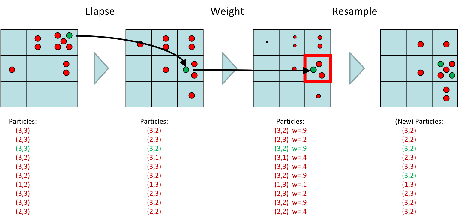
Particle Filtering: Elapse Time
- Each particle is moved by sampling its next position from the transition model \[x' = sample(P(X'|x))\]
- This is like prior sampling – samples’ frequencies reflect the transition probabilities
- Here, most samples move clockwise, but some move in another direction or stay in place
- This captures the passage of time
- If enough samples, close to exact values before and after (consistent)

Particle Filtering: Observe
- Slightly trickier:
- Do not sample observation, fix it
- Similar to likelihood weighting, downweight samples based on the evidence \begin{equation} \begin{aligned} w(x) &= P(e|x) \nonumber \\ B(X) &\propto P(e|X)B'(X) \nonumber \end{aligned} \end{equation}
- As before, the probabilities don’t sum to one, since all have been downweighted (in fact they now sum to ($N$ times) an approximation of $P(e)$)

Particle Filtering: Resample
- Rather than tracking weighted samples, we resample
- $N$ times, we choose from our weighted sample distribution (i.e. draw with replacement)
- This is equivalent to renormalizing the distribution
- Now the update is complete for this time step, continue with the next one

Summary: Particle Filtering
- Particles: track samples of states rather than an explicit distribution
Particle Filtering Applications
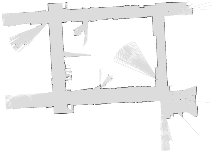
Robot Localization
- In robot localization:
- We know the map, but not the robot’s position
- Observations may be vectors of range finder readings
- State space and readings are typically continuous (works basically like a very fine grid) and so we cannot store $B(X)$
- Particle filtering is a main technique

Particle Filter Localization (Sonar)
Robot Mapping
- SLAM: Simultaneous Localization And Mapping
- We do not know the map or our location
- State consists of position AND map
- Main techniques: Kalman filtering (Gaussian HMMs) and particle methods
Particle Filter SLAM - Video 1
Particle Filter SLAM - Video 2
Dynamic Bayes Net
Dynamic Bayes Nets (DBNs)
- We want to track multiple variables over time, using multiple sources of evidence
- Idea: Repeat a fixed Bayes net structure at each time
- Variables from time t can condition on those from $t-1$
- Dynamic Bayes nets are a generalization of HMMs


Exact Inference in DBNs
- Variable elimination applies to dynamic Bayes nets
- Procedure: "unroll" the network for T time steps, then eliminate variables until $P(X_T|e_{1:T})$ is computed
- Online belief updates: Eliminate all variables from the previous time step; store factors for current time only


DBN Particle Filters
- A particle is a complete sample for a time step
- Initialize: Generate prior samples for the t=1 Bayes net
- Example particle: $G_2^a = (3,3)$ $G_1^b=(5,3)$
- Elapse time: Sample a successor for each particle
- Example successor: $G_2^a = (2,3)$ $G_2^b=(6,3)$
- Observe: Weight each entire sample by the likelihood of the evidence conditioned on the sample
- Likelihood: $P(E_1^a|G_1^a) \times P(E_1^b|G_1^b)$
- Resample: Select prior samples (tuples of values) in proportion to their likelihood
Most Likely Explanation
HMMs: MLE Queries
- HMMs defined by:
- States $X$
- Observations $E$
- Initial distribution: $P(X_1)$
- Transitions: $P(X_t|X_{t-1})$
- Emissions: $P(E_t|X_t)$
- New query: most likely explanation: $\underset{x_{1:t}}{\operatorname{arg max}} P(x_{1:t}|e_{1:t})$
- New method: the Viterbi algorithm
State Trellis
- State trellis: graph of states and transitions over time
- Each arc represents some transition $x_{t-1} \rightarrow x_t$
- Each arc has weight $P(x_t|x_{t-1})P(e_t|x_t)$
- Each path is a sequence of states
- The product of weights on a path is that sequence's probability along with the evidence
- Forward algorithm computes sums of paths, Viterbi computes best paths

Forward/Viterbi Algorithms
Speech Recognition
Speech Recognition in Action
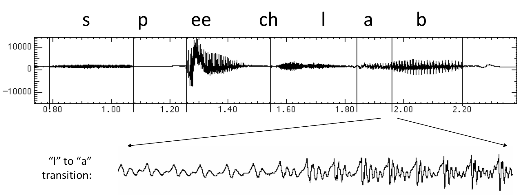
Basics of Speech
- Speech input is an acoustic waveform.
Spectral Analysis
- Frequency gives pitch; amplitude gives volume
- Sampling at ~8 kHz (phone), ~16 kHz (mic) (kHz=1000 cycles/sec)
- Fourier transform of wave displayed as a spectrogram
- Darkness indicates energy at each frequency


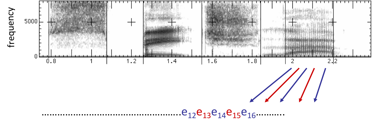
Acoustic Feature Sequence
- Time slices are translated into acoustic feature vectors ($\sim$39 real numbers per slice)
- These are the observations $E$, now we need the hidden states $X$
Speech State Space
- HMM Specification
- $P(E|X)$ encodes which acoustic vectors are appropriate for each phoneme (each kind of sound)
- $P(X|X')$ encodes how sounds can be strung together
- State Space
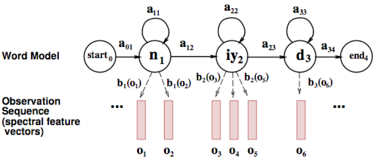
- We will have one state for each sound in each word
- Mostly, states advance sound by sound
- Build a little state graph for each word and chain them together to form the state space $X$
States in a Word
Transitions with a Bigram Model

Decoding
- Finding the words given the acoustics is an HMM inference problem
- Which state sequence $x_{1:T}$ is most likely given the evidence $e_{1:T}$? \[x^*_{1:T} = \underset{x_{1:T}}{\operatorname{arg max}}P(x_{1:T}|e_{1:T}) = \underset{x_{1:T}}{\operatorname{arg max}} P(x_{1:T},e_{1:T})\]
- From the sequence $x$, we can simply read off the words
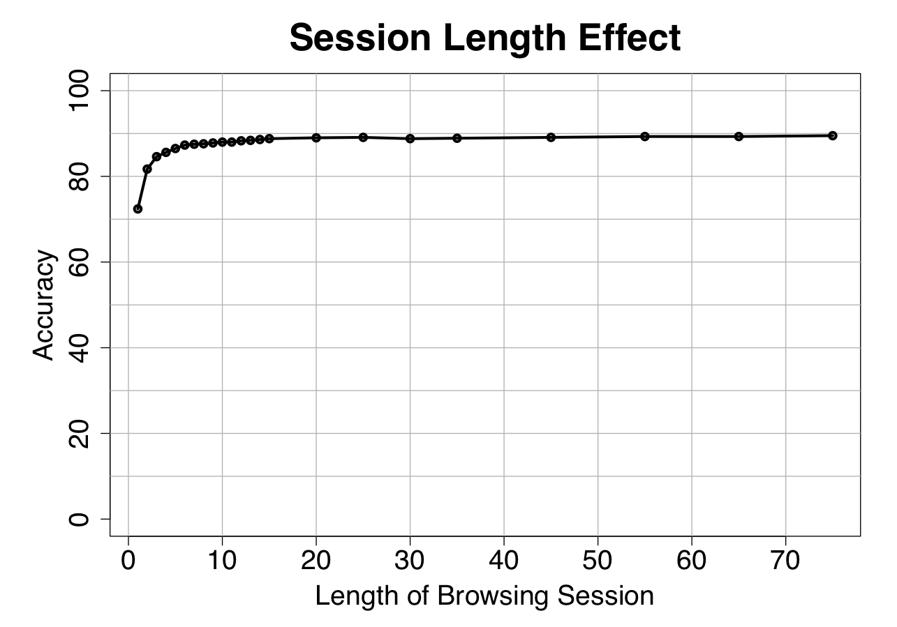
Results
Q & A