Backpropagation
CSE 849: Deep Learning
Today
- Chain Rule
- Computational Graphs
- Backpropagation
Overview
- Given a neural network, our goal is to learn the optimal parameters.
- Backpropagation is one of the central tool necessary for this purpose.
- It is an algorithm to efficiently compute gradients.
- It is an instance of reverse-mode automatic differentiation, a more broadly applicable tool for computing gradients.
- Salient Features of Backpropagation are:
- Chain Rule
- Gradient Caching
Derivatives of Functions
$$ \begin{align} z &= wx + b & y &= \sigma(z) & \mathcal{L} &= \frac{1}{2}(y-t)^2 \nonumber \end{align} $$- Compute Derivatives using Calculus:
$$
\begin{eqnarray}
\frac{\partial \mathcal{L}}{\partial w} &=& \nonumber \\
&=& \nonumber \\
&=& \nonumber \\
&=& \nonumber \\
&=& \nonumber
\end{eqnarray}
$$
$$
\begin{eqnarray}
\frac{\partial \mathcal{L}}{\partial b} &=& \nonumber \\
&=& \nonumber \\
&=& \nonumber \\
&=& \nonumber \\
&=& \nonumber
\end{eqnarray}
$$
Derivatives of Functions
$$ \begin{align} z &= wx + b & y &= \sigma(z) & \mathcal{L} &= \frac{1}{2}(y-t)^2 \nonumber \end{align} $$- Compute Derivatives using Calculus:
$$
\begin{eqnarray}
\frac{\partial \mathcal{L}}{\partial w} &=& \frac{\partial}{\partial w} \left[\frac{1}{2}(\sigma(wx+b)-t)^2\right] \nonumber \\
&=& \frac{1}{2}\frac{\partial}{\partial w} (\sigma(wx+b)-t)^2 \nonumber \\
&=& (\sigma(wx+b)-t)\frac{\partial}{\partial w} (\sigma(wx+b)-t) \nonumber \\
&=& (\sigma(wx+b)-t)\sigma'(wx+b)\frac{\partial}{\partial w} (wx+b) \nonumber \\
&=& (\sigma(wx+b)-t)\sigma'(wx+b)x \nonumber
\end{eqnarray}
$$
$$
\begin{eqnarray}
\frac{\partial \mathcal{L}}{\partial b} &=& \frac{\partial}{\partial w} \left[\frac{1}{2}(\sigma(wx+b)-t)^2\right] \nonumber \\
&=& \frac{1}{2}\frac{\partial}{\partial b} (\sigma(wx+b)-t)^2 \nonumber \\
&=& (\sigma(wx+b)-t)\frac{\partial}{\partial b} (\sigma(wx+b)-t) \nonumber \\
&=& (\sigma(wx+b)-t)\sigma'(wx+b)\frac{\partial}{\partial b} (wx+b) \nonumber \\
&=& (\sigma(wx+b)-t)\sigma'(wx+b) \nonumber
\end{eqnarray}
$$
- What are the disadvantages of this approach?
Chain Rule
Univariate Chain Rule
- Univariate Chain Rule: If $f(x)$ and $x(t)$ are two univariate functions, then $$ \begin{equation} \frac{\partial}{\partial t}f(x(t)) = \frac{\partial f}{\partial x}\frac{\partial x}{\partial t} \end{equation} $$
Univariate Chain Rule Example
- Forward Pass: $$ \begin{eqnarray} z &=& wx + b \nonumber \\ y &=& \sigma(z) \nonumber \\ \mathcal{L} &=& \frac{1}{2}(y-t)^2 \nonumber \end{eqnarray} $$
- Computing Derivatives using Chain Rule: $$ \begin{eqnarray} \mathcal{L}' &=& \nonumber \\ y' &=& \nonumber \\ z' &=& \nonumber \\ w' &=& \nonumber \\ b' &=& \nonumber \end{eqnarray} $$
Univariate Chain Rule Example
- Forward Pass: $$ \begin{eqnarray} z &=& wx + b \nonumber \\ y &=& \sigma(z) \nonumber \\ \mathcal{L} &=& \frac{1}{2}(y-t)^2 \nonumber \end{eqnarray} $$
- Computing Derivatives using Chain Rule: $$ \begin{eqnarray} \mathcal{L}' &=& 1 \nonumber \\ y' &=& y - t \nonumber \\ z' &=& y'\sigma'(z) \nonumber \\ w' &=& z'x \nonumber \\ b' &=& z' \nonumber \end{eqnarray} $$
- Remember, the goal is not to obtain closed-form solutions, but to be able to write a program that efficiently computes the derivatives.
Univariate Chain Rule
- We can represent the computations using a computational graph.
- Nodes represent all the inputs and computed quantities.
- Edges represent which nodes are computed directly as a function of which other nodes.

Multivariate Chain Rule
- Problem: what if the computation graph has a fan-out $> 1$
- This requires the multivariate Chain Rule.

$$
\begin{eqnarray}
z &=& wx + b \nonumber \\
y &=& \sigma(z) \nonumber \\
\mathcal{L} &=& \frac{1}{2}(y-t)^2 \nonumber \\
\mathcal{R} &=& \frac{1}{2}w^2 \nonumber \\
\mathcal{L}_{reg} &=& \mathcal{L} + \lambda\mathcal{R} \nonumber
\end{eqnarray}
$$

$$
\begin{eqnarray}
z_l &=& \sum_j w_{lj}x_j + b_l \nonumber \\
y_k &=& \frac{e^{z_k}}{\sum_l e^{z_l}} \nonumber \\
\mathcal{L} &=& -\sum_{k}t_k\log y_k \nonumber
\end{eqnarray}
$$
Multivariate Chain Rule
- Suppose we have a function $f(x,y)$ and functions $x(t)$ and $y(t)$.
- All the variables here are scalar-valued.
$$
\begin{equation}
\frac{d}{dt}f(x(t),y(t)) = \frac{\partial f}{\partial x}\frac{dx}{dt} + \frac{\partial f}{\partial y}\frac{dy}{dt}
\end{equation}
$$

Multivariate Chain Rule Example
- Forward Pass: $$ \begin{eqnarray} f(x,y) &=& y + \exp(xy) \nonumber \\ x(t) &=& \cos(t) \nonumber \\ y(t) &=& t^2 \nonumber \end{eqnarray} $$
- Computing Derivatives: $$ \begin{eqnarray} \frac{\partial f}{\partial t} &=& \nonumber \\ \end{eqnarray} $$
Multivariate Chain Rule Example
- Forward Pass: $$ \begin{eqnarray} f(x,y) &=& y + \exp(xy) \nonumber \\ x(t) &=& \cos(t) \nonumber \\ y(t) &=& t^2 \nonumber \end{eqnarray} $$
- Computing Derivatives: $$ \begin{eqnarray} \frac{\partial f}{\partial t} &=& \frac{\partial f}{\partial x}\frac{\partial x}{\partial t} + \frac{\partial f}{\partial y}\frac{\partial y}{\partial t} \nonumber \\ &=& (y\exp(xy))\cdot(-\sin(t)) \nonumber \\ && + (1+x\exp(xy))\cdot(2t) \nonumber \end{eqnarray} $$
Backpropagation
Multivariate Chain Rule
- In the context of backpropagation:
- In our notation: $$ \begin{equation} t' = x'\frac{dx}{dt} + y'\frac{dy}{dt} \end{equation} $$

Patterns in Gradient Flow


Univariate Backpropagation
- Example: univariate least squares regression
- Forward Pass:
- Backward Pass:
$$
\begin{eqnarray}
\mathcal{L}'_{reg} &=& 1 \nonumber \\
\mathcal{R}' &=& \mathcal{L}_{reg}'\frac{d \mathcal{L}}{d \mathcal{R}} \nonumber \\
&=& \mathcal{L}_{reg}'\lambda \nonumber \\
\mathcal{L}' &=& \mathcal{L}_{reg}'\frac{d \mathcal{L}}{d \mathcal{L}} \nonumber \\
&=& \mathcal{L}_{reg}' \nonumber \\
y' &=& \mathcal{L}'\frac{d \mathcal{L}}{dy} \nonumber \\
&=& \mathcal{L}'(y-t) \nonumber \\
\end{eqnarray}
$$
$$
\begin{eqnarray}
z' &=& y'\frac{dy}{dz} \nonumber \\
&=& y'\sigma'(z) \nonumber \\
w' &=& z'\frac{\partial z}{\partial w}+\mathcal{R}'\frac{d \mathcal{R}}{dw} \nonumber \\
&=& z'x + \mathcal{R}'w \nonumber \\
b' &=& z'\frac{\partial z}{\partial b} \nonumber \\
&=& z'
\end{eqnarray}
$$
Multivariate Backpropagation
- Example: Multilayer Perception (multiple outputs)

- Forward Pass:
- Backward Pass:
Vector Form
- Computation graphs showing individual units are cumbersome.
- As you might imagine, we typically draw graphs over vectorized variables.
- We pass messages back analogous to the ones for scalar-valued nodes.

Vector Form
- Consider this computation graph:
- Backprop rules: $$ \begin{equation} z_{j}' = \sum_{k}y_k'\frac{\partial y_k}{\partial z_j} \mbox{ or } \mathbf{z}' = \frac{\partial \mathbf{y}^T}{\partial \mathbf{z}}\mathbf{y}' \end{equation} $$
- where $\frac{\partial \mathbf{y}}{\partial \mathbf{z}}$ is the Jacobian matrix: $\mathbf{J} = \frac{\partial \mathbf{y}}{\partial \mathbf{x}} = \begin{bmatrix} \frac{\partial y_1}{\partial x_1} & \dots & \frac{\partial y_1}{\partial x_n} \\\ \vdots & \ddots & \vdots \\\ \frac{\partial y_n}{\partial x_1} & \dots & \frac{\partial y_n}{\partial x_n} \end{bmatrix}$

MLP Backpropagation
- Example: Multilayer Perception (vector form)
- Forward Pass:
- Backward Pass:
Backpropagation Implementation: Modular API
    class ComputationalGraph(object):
      # ...
      def forward(inputs):
        # 1. [pass inputs to input gates]
        # 2. forward the computational graph
        for gate in self.graph_nodes_topologically_sorted():
          gate.forward()
        return loss # final gate in the graph outputs the loss
      def backward(loss):
        for gate in reversed(self.graph_nodes_topologically_sorted()):
          gate.backward() # chain rule applied
        return input_gradients
Backpropagation: PyTorch Example
    class Multiply(torch.autograd.Function):
      @staticmethod
      def forward(ctx, x, y):
        ctx.save_for_backward(x,y)
        z = x * y
        return z
      @staticmethod
      def backward(ctx, grad_z):
        x, y = ctx.saved_tensors
        grad_x = y * grad_z # dz/dx * dL/dz
        grad_y = x * grad_z # dz/dy * dL/dz
        return grad_x, grad_y
Caching Gradients
$$ \begin{equation} \frac{\partial l}{\partial \mathbf{\theta}} = \left[\frac{\partial l}{\mathbf{W}_1},\frac{\partial l}{b_1},\dots,\frac{\partial l}{\mathbf{W}_L},\frac{\partial l}{b_L} \right] \nonumber \end{equation} $$ $$ \begin{eqnarray} f(\mathbf{x}) &=& \mathbf{b}+\mathbf{W}\mathbf{x} \nonumber \\ o(\mathbf{x}) &=& g^L\left(f^L\left(g^{L-1}\left(f^{L-1}\left(\dots\right)\right)\right)\right) \nonumber \end{eqnarray} $$- $\frac{\partial l}{\partial W^L_{ij}} = $
- $\frac{\partial l}{\partial W^{L-1}_{ij}} = $
Caching Gradients
$$ \begin{equation} \frac{\partial l}{\partial \mathbf{\theta}} = \left[\frac{\partial l}{\mathbf{W}_1},\frac{\partial l}{b_1},\dots,\frac{\partial l}{\mathbf{W}_L},\frac{\partial l}{b_L} ]\right] \nonumber \end{equation} $$ $$ \begin{eqnarray} f(\mathbf{x}) &=& \mathbf{b}+\mathbf{W}\mathbf{x} \nonumber \\ o(\mathbf{x}) &=& g^L\left(f^L\left(g^{L-1}\left(f^{L-1}\left(\dots\right)\right)\right)\right) \nonumber \end{eqnarray} $$- $\frac{\partial l}{\partial W^L_{ij}} = \frac{\partial l}{\partial o(\mathbf{x})}\frac{\partial o(\mathbf{x})}{\partial g^L}\frac{\partial g^L}{\partial f^L}\frac{\partial f^L}{\partial W^L_{ij}}$
- $\frac{\partial l}{\partial W^{L-1}_{ij}} = \frac{\partial l}{\partial o(\mathbf{x})}\frac{\partial o(\mathbf{x})}{\partial g^L}\frac{\partial g^L}{\partial f^L}\frac{\partial f^L}{\partial g^{L-1}}\frac{\partial g^{L-1}}{\partial f^{L-1}}\frac{\partial f^{L-1}}{\partial W^{L-1}_{ij}}$
Computational Cost
- Computational cost of forward pass: one add-multiply operation per weight $$ z_i = \sum_j w^{(1)}_{ij}x_j + b^{(1)}_i $$
- Computational cost of backward pass: two add-multiply operations per weight $$w^{(2)}_{ki} = y_k' h_i$$ $$h_{i}' = \sum_k y_k' w^{(2)}_{ki}$$
- Rule of thumb: the backward pass is about as expensive as two forward passes.
- For a multilayer perceptron, this means the cost is linear in the number of layers, quadratic in the number of units per layer.
Q & A

MLP Gradients (Optional)
Recap: Multilayer Neural Network
- Could have $L$ hidden layers:
- layer pre-activation for $k>0$ ($\mathbf{h}^{(0)}(\mathbf{x})=\mathbf{x}$) $\mathbf{a}^{(k)}(\mathbf{x}) = \mathbf{b}^{(k)} + \mathbf{W}^{(k)}\mathbf{h}^{(k-1)}(\mathbf{x})$
- hidden layer activation ($k$ from 1 to $L$): $\mathbf{h}^{(k)}(\mathbf{x}) = \mathbf{g}(\mathbf{a}^{(k)}(\mathbf{x}))$
- output layer activation ($k=L+1$): $\mathbf{h}^{(L+1)}(\mathbf{x}) = \mathbf{o}(\mathbf{a}^{(L+1)}(\mathbf{x})) = f(\mathbf{x})$

Loss Function
- Maximum Likelihood Estimate: $$ \mathbf{\theta}^* = \underset{\theta}{\operatorname{arg max}}\prod_i p(y_i=c|\mathbf{x}_i) $$
- Classification: $$ l = l(\mathbf{x},\mathbf{\theta};y) = \sum_i -\log f(\mathbf{x}_i)_y $$
Output Layer Gradient
- Partial Derivative: \begin{equation} \frac{\partial}{\partial f(\mathbf{x})_c} -\log f(\mathbf{x})_y = -\frac{1_{y=c}}{f(\mathbf{x})_y} \nonumber \end{equation}
- Gradient: \begin{eqnarray} && \nabla_{f(\mathbf{x})} -\log f(\mathbf{x})_y \nonumber \\ &=& \frac{-1}{f(\mathbf{x})_y} \begin{bmatrix} 1_{y=0} \\ \vdots \\ 1_{y=C-1} \end{bmatrix} \nonumber \\ &=& \frac{-e(y)}{f(\mathbf{x})_y} \nonumber \end{eqnarray}
Output Layer Gradient Continued...
- Partial Derivative: $$ \begin{eqnarray} && \frac{\partial}{\partial a^{(L+1)}(\mathbf{x})_c} -\log f(\mathbf{x})_y \nonumber \\ &=& -(1_{y=c}-f(\mathbf{x})_c) \nonumber \end{eqnarray} $$
- Gradient: \begin{eqnarray} && \nabla_{a^{(L+1)}(\mathbf{x})} -\log f(\mathbf{x})_y \nonumber \\ &=& -(\mathbf{e}(y)-f(\mathbf{x})) \nonumber \end{eqnarray}
Hidden Layer Gradient
- Partial Derivative: $$ \begin{eqnarray} && \frac{\partial}{\partial h^{(k)}(\mathbf{x})_j}-\log f(\mathbf{x})_y \nonumber \\ &=& \sum_i \frac{\partial-\log f(\mathbf{x})_y}{\partial a^{(k+1)}(\mathbf{x})_i}\frac{\partial a^{(k+1)}(\mathbf{x})_i}{\partial h^{(k)}(\mathbf{x})_j} \nonumber \\ &=& \sum_i \frac{\partial-\log f(\mathbf{x})_y}{\partial a^{(k+1)}(\mathbf{x})_i}W^{k+1}_{i,j} \nonumber \\ &=& \left(\mathbf{W}^{k+1}_{.,j}\right)^T\left(\nabla_{a^{(k+1)}(\mathbf{x})}-\log f(\mathbf{x})_y\right) \nonumber \end{eqnarray} $$
Activation Function Gradient
- Partial Derivative: $$ \begin{eqnarray} && \frac{\partial}{\partial a^{(k)}(\mathbf{x})_j}-\log f(\mathbf{x})_y \nonumber \\ &=& \frac{\partial -\log f(\mathbf{x})_y}{\partial h^{(k)}(\mathbf{x})_j}\frac{\partial h^{(k)}(\mathbf{x})_j}{\partial a^{(k)}(\mathbf{x})_j} \nonumber \\ &=& \frac{\partial}{\partial h^{(k)}(\mathbf{x})_j}g'\left(a^{(k)}(\mathbf{x})_j\right) \nonumber \\ &=& (\nabla_{h^{(k)}(\mathbf{x})}-\log f(\mathbf{x})_y) \odot [\dots,g'\left(a^{(k)}(\mathbf{x})_j\right),\dots] \nonumber \end{eqnarray} $$
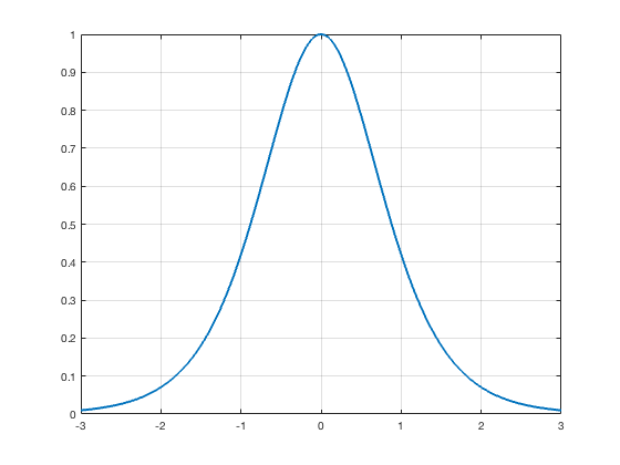
Linear Activation
$$g(x) = x$$
$$\nabla g(x) = 1$$
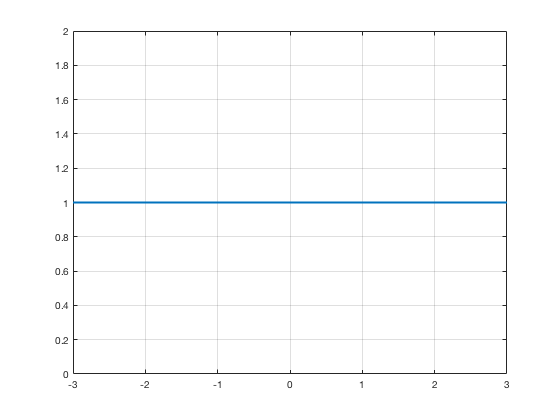
Sigmoid Activation
$$g(x) = \frac{1}{1+e^{-x}}$$
$$\nabla g(x) = g(x)\left(1-g(x)\right)$$
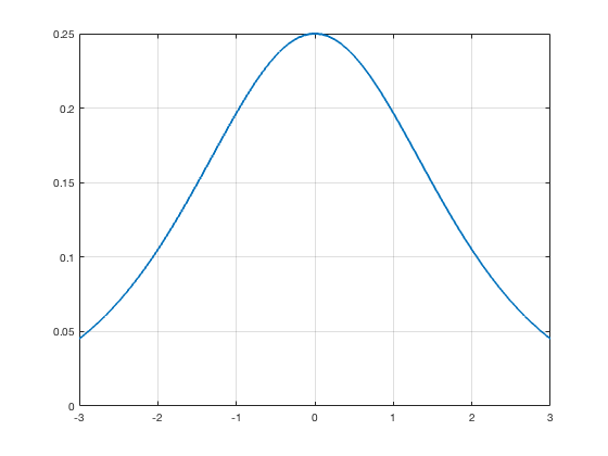
Tanh Activation
$$g(x) = \frac{e^{x}-e^{-x}}{e^{x}+e^{-x}}$$
$$\nabla g(x) = 1-g(x)^2$$
Rectified Linear Unit Activation
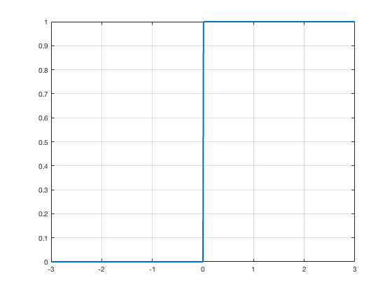
$$g(x) = max(0,x)$$
$$\nabla g(x) = \begin{cases} 0 & \quad \text{for } x < 0 \\ 1 & \quad \text{for } x > 0 \end{cases}$$
Gradient of Parameters
- Partial Derivative (weights): $$ \begin{eqnarray} && \frac{\partial}{\partial W^{(k)}_{i,j}}-\log f(\mathbf{x})_y \nonumber \\ &=& \frac{\partial -\log f(\mathbf{x})_y}{\partial a^{(k)}(\mathbf{x})_i}\frac{\partial a^{(k)}(\mathbf{x})_i}{\partial W^{(k)}_{i,j}} \nonumber \\ &=& \frac{\partial -\log f(\mathbf{x})_y}{\partial a^{(k)}(\mathbf{x})_i}h_j^{(k-1)}(\mathbf{x}) \nonumber \\ &=& \left(\nabla_{\mathbf{a}^(k)}(\mathbf{x})-\log f(\mathbf{x})_y\right) \mathbf{h}^{(k-1)}(\mathbf{x})^T \nonumber \end{eqnarray} $$
Gradient of Parameters
- Partial Derivative (biases): $$ \begin{eqnarray} && \frac{\partial}{\partial b^{(k)}_{i}}-\log f(\mathbf{x})_y \nonumber \\ &=& \frac{\partial -\log f(\mathbf{x})_y}{\partial a^{(k)}(\mathbf{x})_i}\frac{\partial a^{(k)}(\mathbf{x})_i}{\partial b^{(k)}_{i}} \nonumber \\ &=& \frac{\partial -\log f(\mathbf{x})_y}{\partial a^{(k)}(\mathbf{x})_i} \nonumber \\ &=& \left(\nabla_{\mathbf{a}^(k)}(\mathbf{x})-\log f(\mathbf{x})_y\right) \nonumber \end{eqnarray} $$
Backpropagation Algorithm
- Assuming Forward Propagation is already done.
- compute output gradient (before activation) $$ \nabla_{\mathbf{a}^{(L+1)}(\mathbf{x})} -\log f(\mathbf{x})_y \Longleftarrow -(\mathbf{e}(y)-\mathbf{f}(\mathbf{x})) $$
- for $k$ from $L+1$ to 1
- compute gradients of hidden layer parameter $$ \begin{eqnarray} \nabla_{\mathbf{W}^{(k)}} -\log f(\mathbf{x})_y &\Longleftarrow& (\nabla_{\mathbf{a}^{(k)}} -\log f(\mathbf{x})_y) \mathbf{h}^{(k-1)}(\mathbf{x})^T \nonumber \\ \nabla_{\mathbf{b}^{(k)}} -\log f(\mathbf{x})_y &\Longleftarrow& \nabla_{\mathbf{a}^{(k)}} -\log f(\mathbf{x})_y \nonumber \end{eqnarray} $$
- compute gradient of hidden layer below $$ \begin{equation} \nabla_{\mathbf{h}^{(k-1)}} -\log f(\mathbf{x})_y \Longleftarrow \mathbf{W}^{(k)^T}\left(\nabla_{\mathbf{a}^{(k)}} -\log f(\mathbf{x})_y\right) \end{equation} $$
- compute gradient of hidden layer below (before activation) $$ \begin{equation} \nabla_{\mathbf{a}^{(k-1)}} -\log f(\mathbf{x})_y \Longleftarrow \left(\nabla_{\mathbf{h}^{(k-1)}} -\log f(\mathbf{x})_y\right) \odot [\dots,g'(a^{(k-1)}(\mathbf{x})_j),\dots] \nonumber \end{equation} $$
Computational Flow Graph: Forward Pass
- Forward propagation: represented as an acyclic flow graph
- Forward propagation: implement in a modular way
- each box is an object with fprop method, computes value of box given its parents
- call fprop method of each box in the right order to yield forward propagation

Computational Flow Graph: Backward Pass
- Each object also has a bprop method
- computes gradient of loss wrt each child
- bprop depends on the bprop of the a box's children
- calling bprop in the reverse order, we get backpropagation
