Interpretability
CSE 849: Deep Learning
Today
- Visualization
- Adversarial Examples
- Style Transfer
Looking Inside a Neural Network

Weights
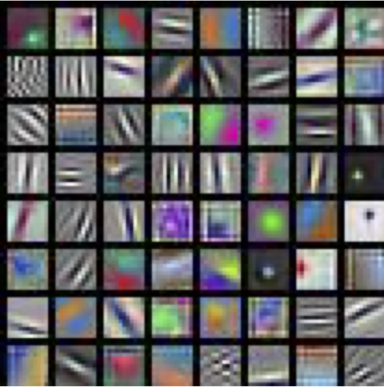
Interpreting Weights: First Layer


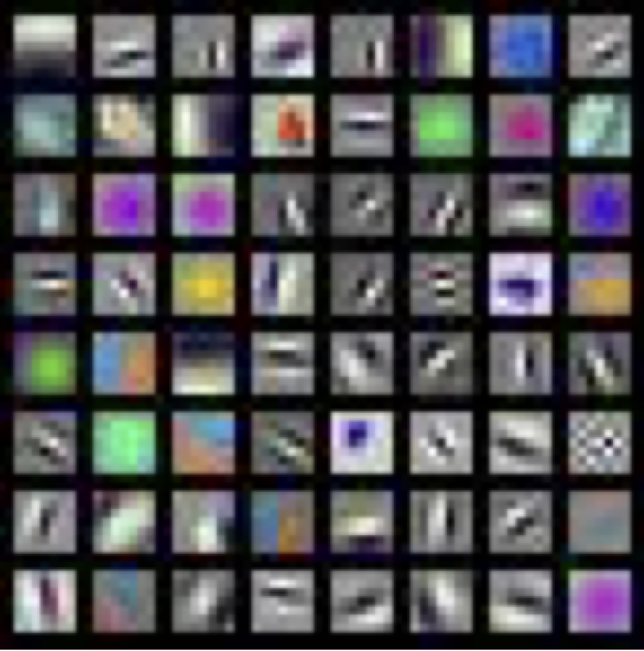
Interpreting Weights: Higher Layer

Features
Interpreting Features
- Last Layer:
- 4096-dimensional feature vector for an image
- layer immediately before the classifier
- Run the network on many images and collect the feature vectors

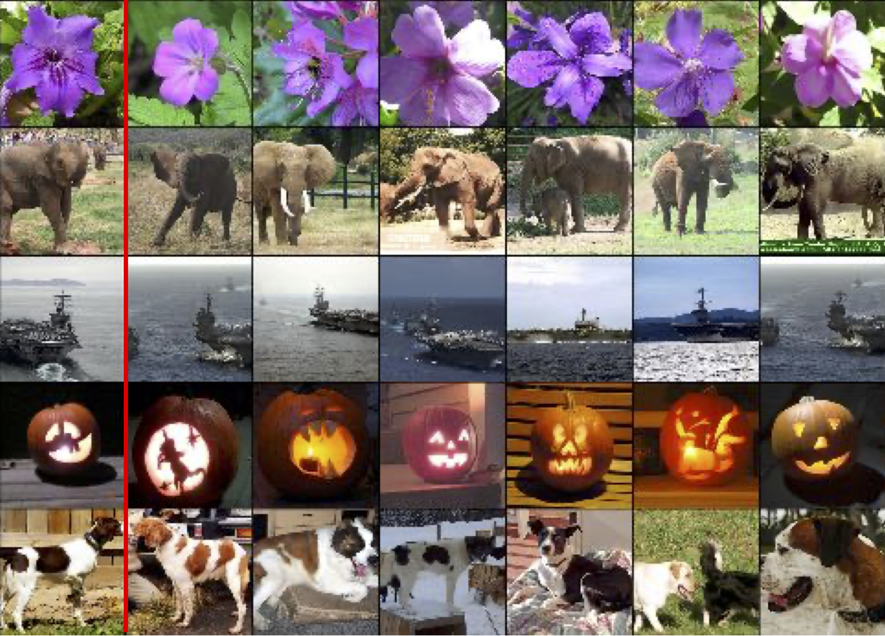
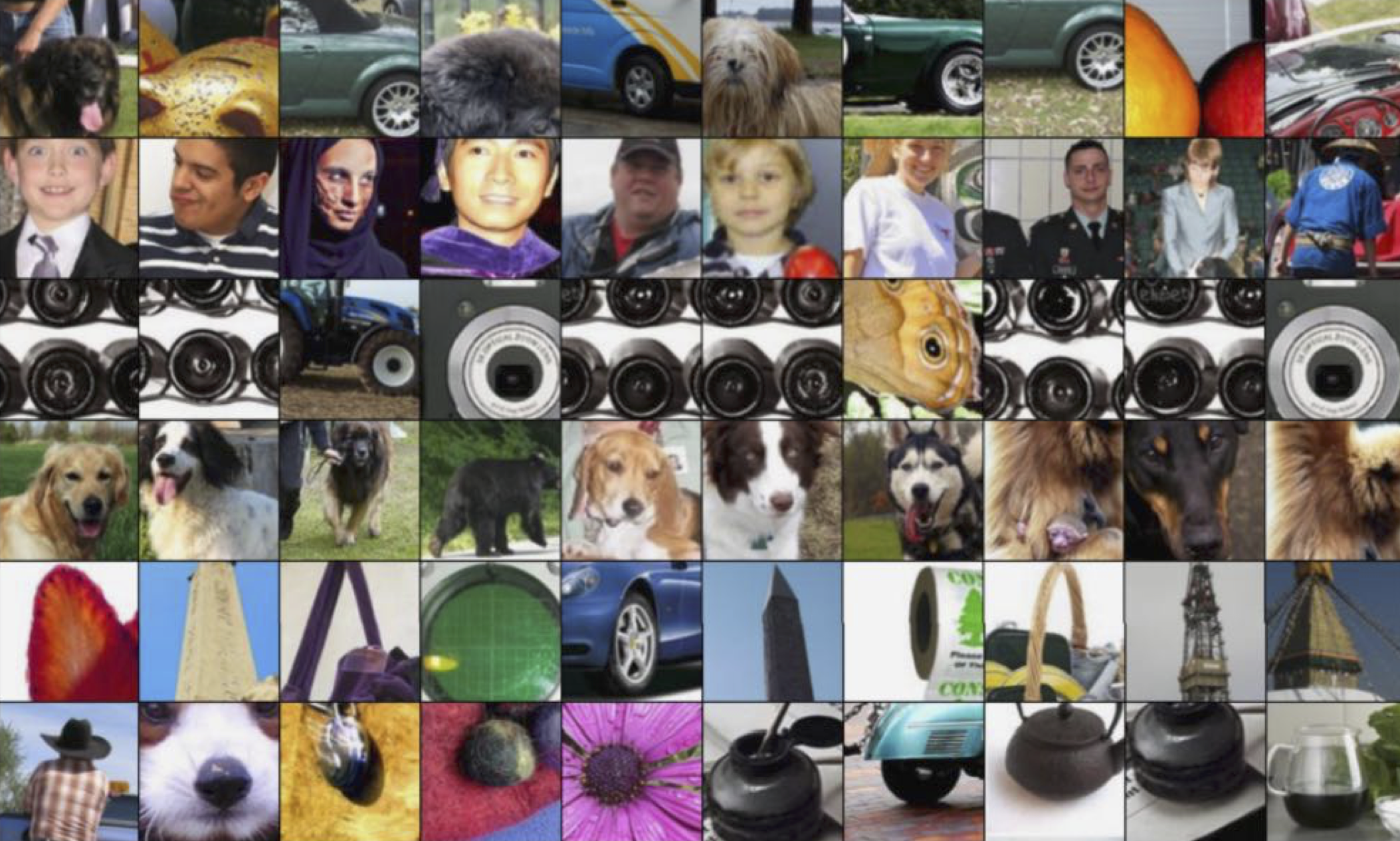
Nearest Neighbors
Dimensionality Reduction
- Visualize the space of feature vectors via dimensionality reduction to 2 dimensions.
- Dimensionality Reduction:
- Principal Component Analysis (PCA)
- More Complex: t-SNE
- Even more complex: DeepMDS
- Van der Maaten and Hinton "Visualizing Data using t-SNE" JMLR 2008
- Gong et.al. "On the Intrinsic Dimensionality of Image Representations" CVPR 2019
Dimensionality Reduction


Activations
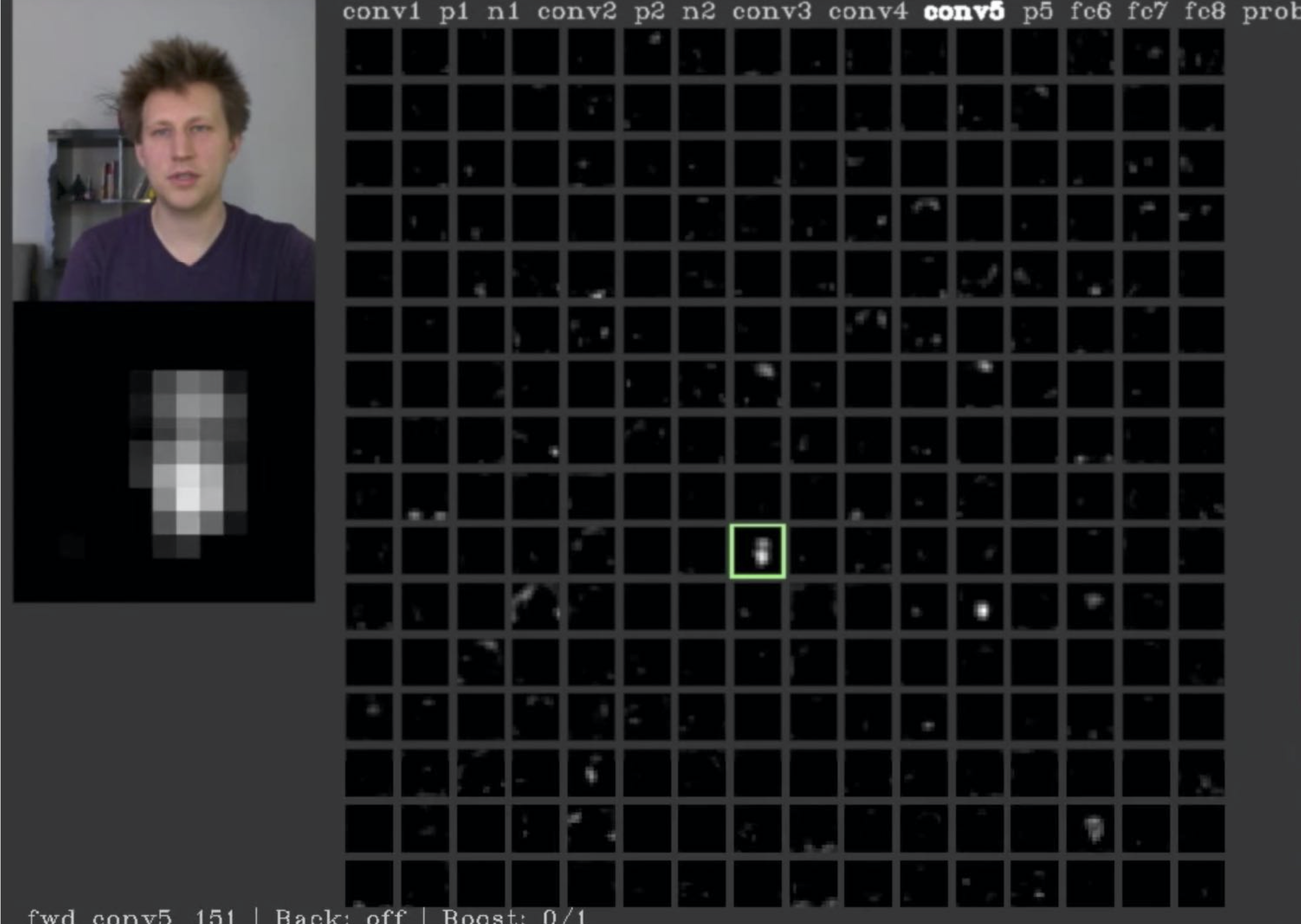
Visualizing Activations
- conv5 feature map is $128\times 13\times 13$; visualize as 128 $13\times 13$ grayscale images.
Maximally Activating Patches
- Pick a layer and a channel; e.g. conv5 is $128\times 13\times 13$, pick channel 17/128
- Run many images through the network, record values of chosen channel
- Visualize image patches that correspond to maximal activations
- Springenberg et.al. "Striving for Simplicity: The All Convolutional Net" ICLR Workshop 2015

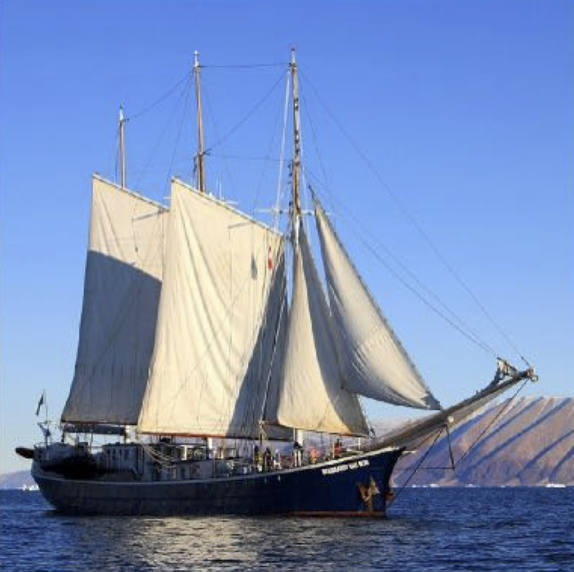
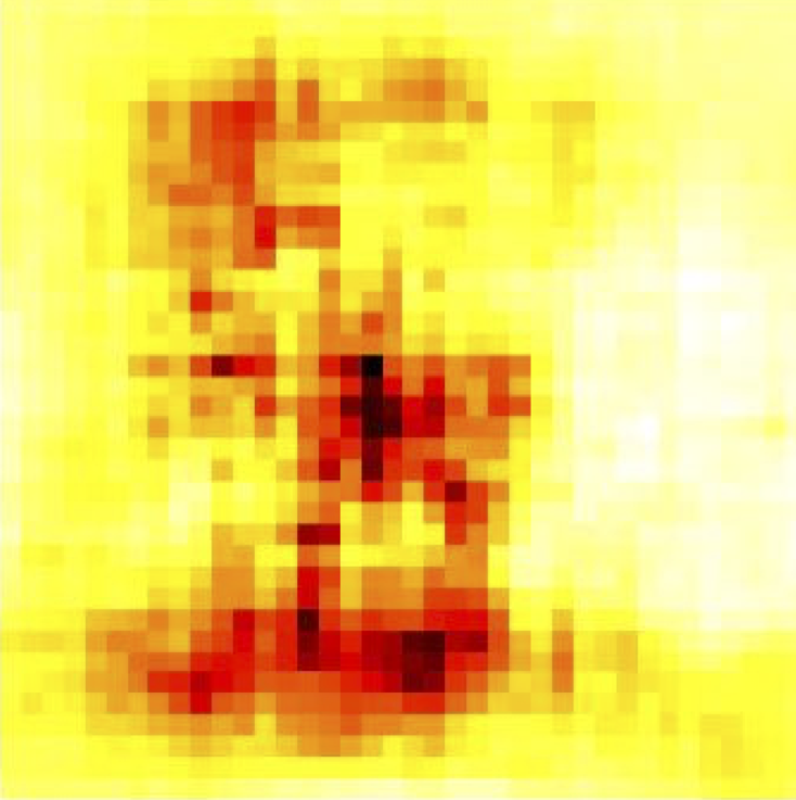
Which Pixels Matter?
- Saliency via Occlusion
- Mask part of the image before feeding to CNN, check how much predicted probabilities change


- Zeiler et.al. "Visualizing and Understanding Convolutional Networks" ECCV 2014


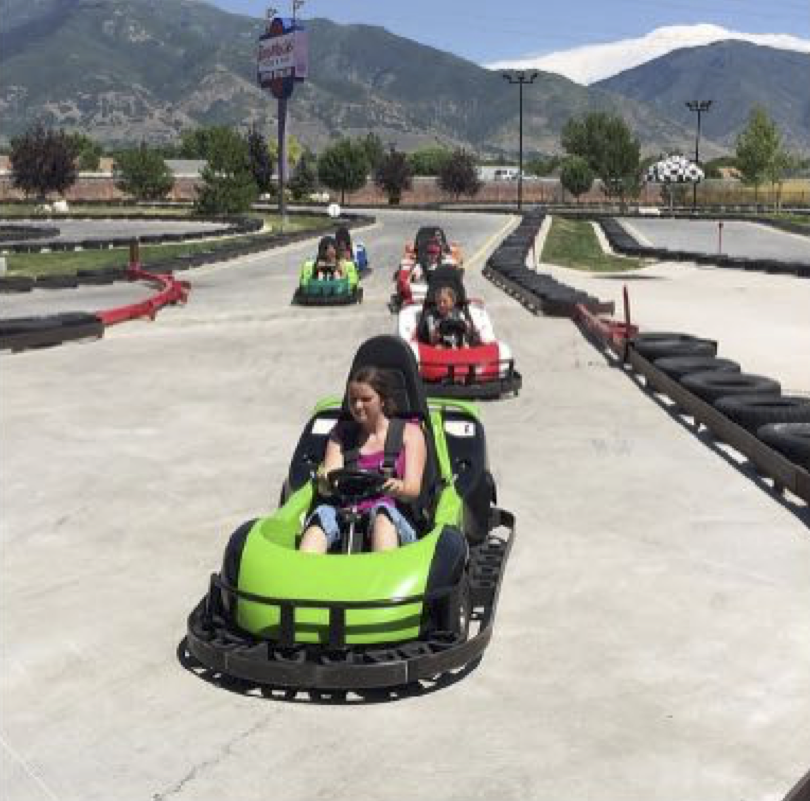
Which Pixels Matter?
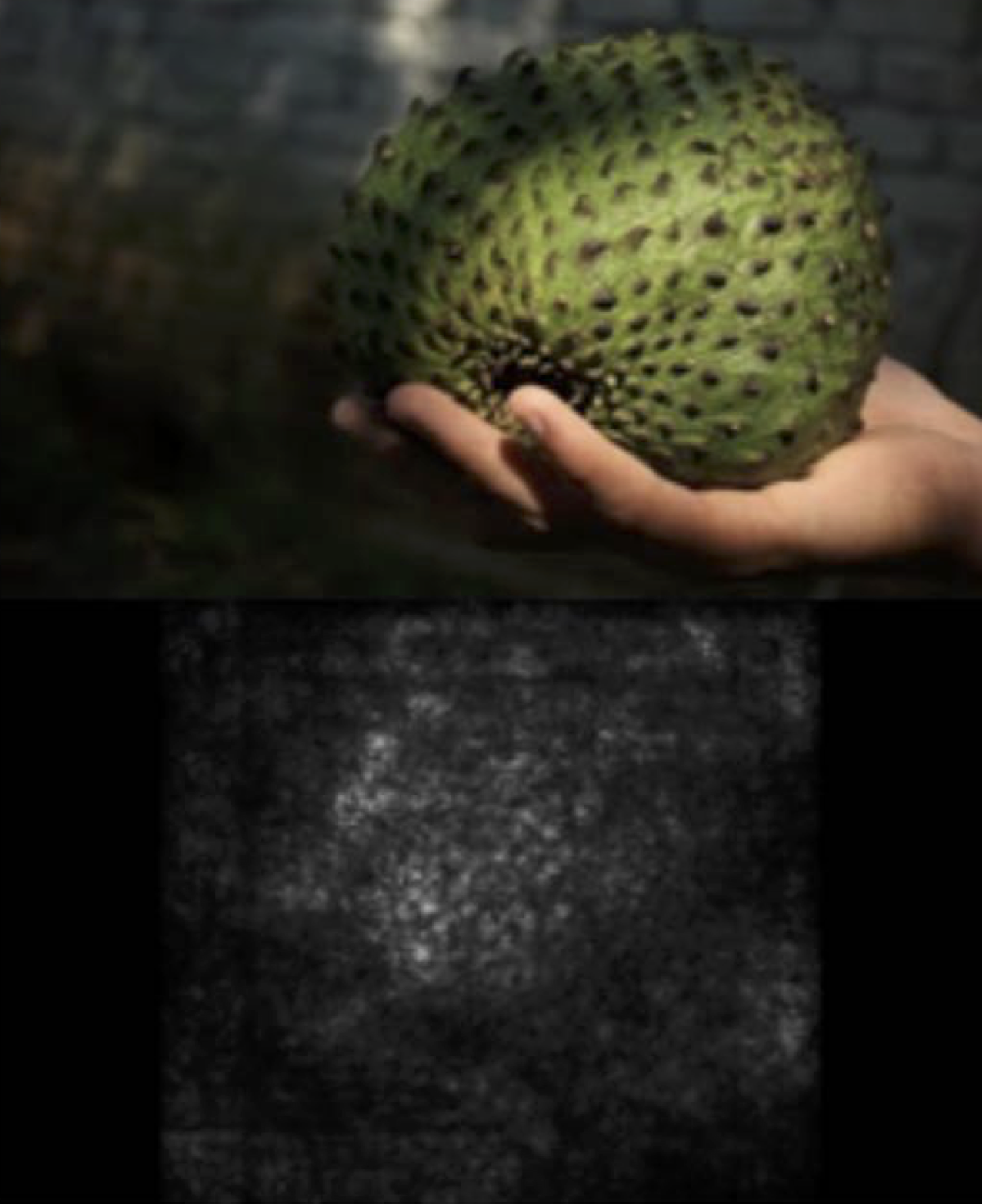
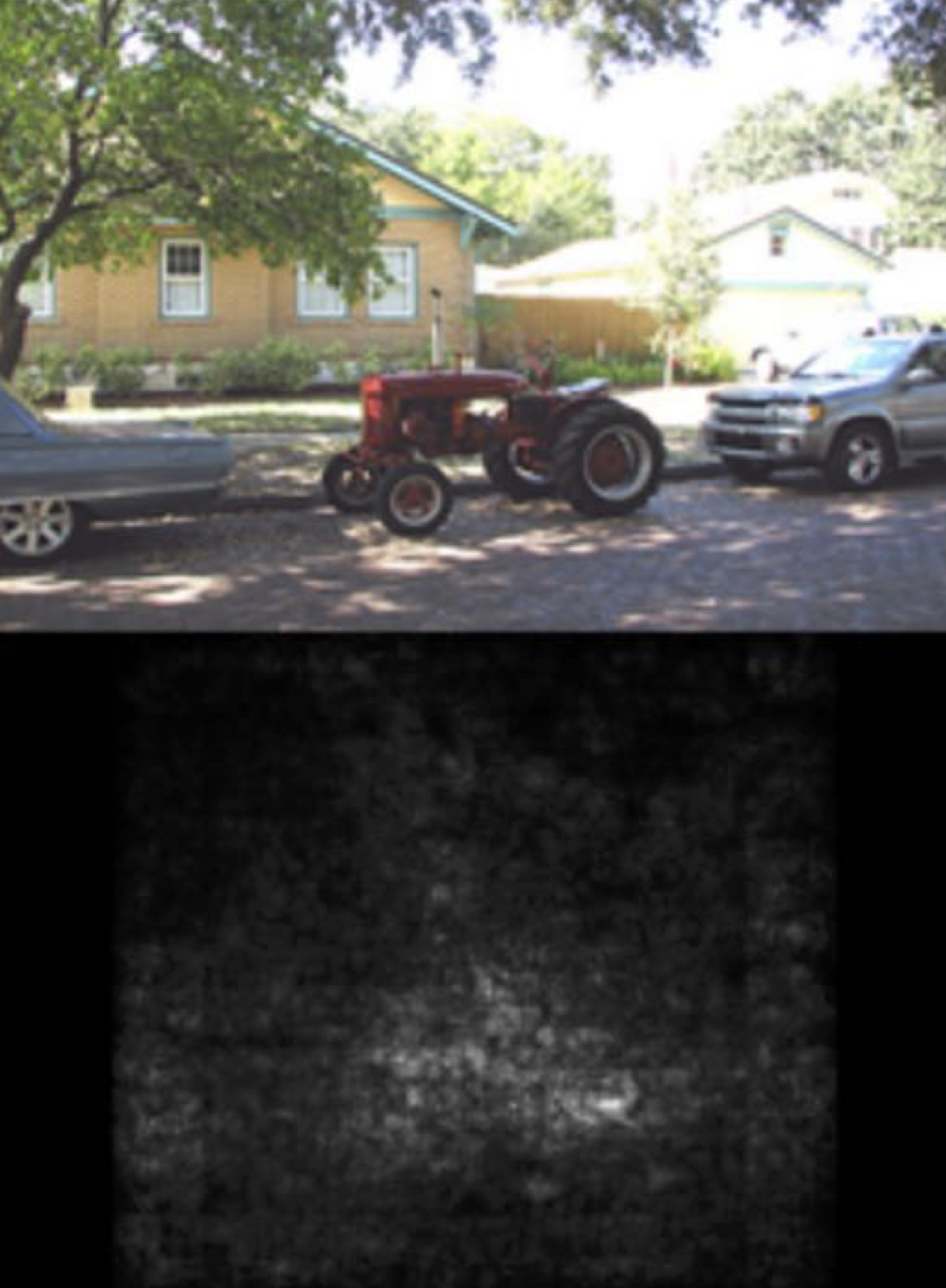
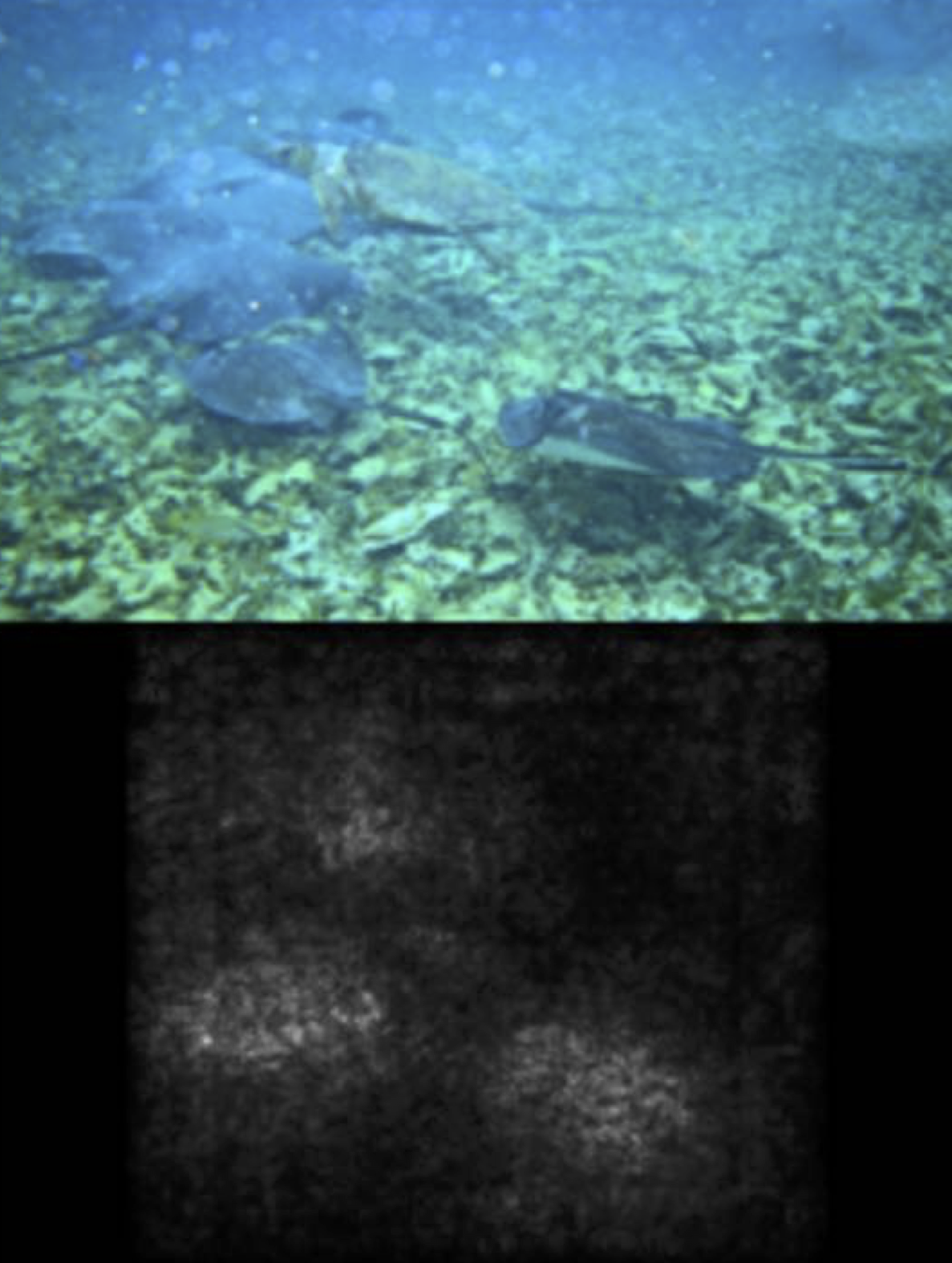
- Saliency via Backpropagation
- Forward pass: Compute probabilities
- Compute gradient of (unnormalized) class score with respect to image pixels, take absolute value and max over RGB channels
- Simonyan et.al. "Deep Inside Convolutional Networks: Visualizing Image Classification Models and Saliency Maps" ICLR Workshop 2014
Saliency via Backprop
- Simonyan et.al. "Deep Inside Convolutional Networks: Visualizing Image Classification Models and Saliency Maps" ICLR Workshop 2014
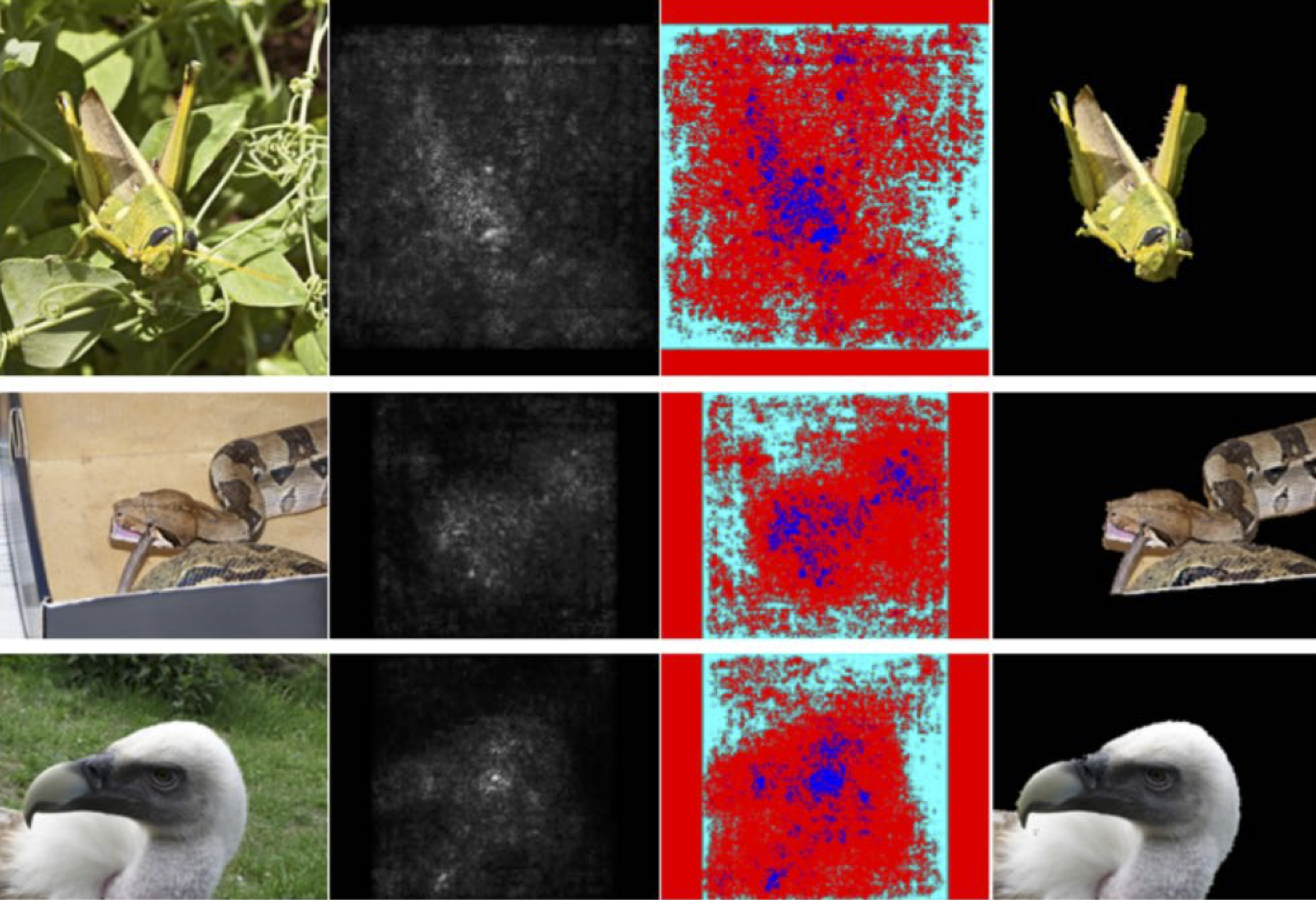
Segmentation from Saliency Maps
Guided Backpropagation
- Guided backprop is a total hack, but useful.
- Do the backward pass as normal, but apply the ReLU nonlinearity to all the activation error signals. $$ \begin{equation} y = \mbox{ReLU}(z) \quad z' = \begin{cases} y' & \quad \text{if } z > 0 \mbox{ and } y' > 0 \\ 0 & \quad \text{otherwise}\end{cases} \end{equation} $$
- Note: this isn’t really the gradient of anything!
- We want to visualize what excites a given unit, not what suppresses it.
Guided Backpropagation Examples


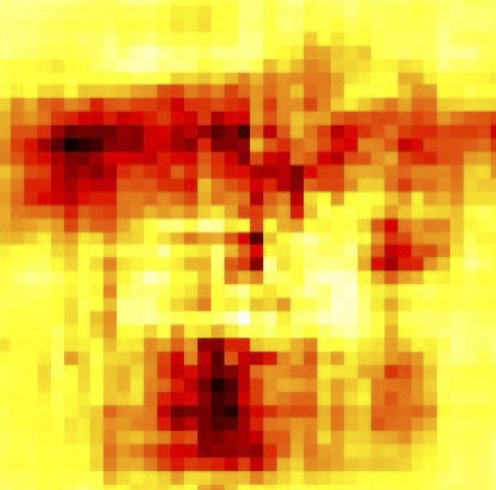
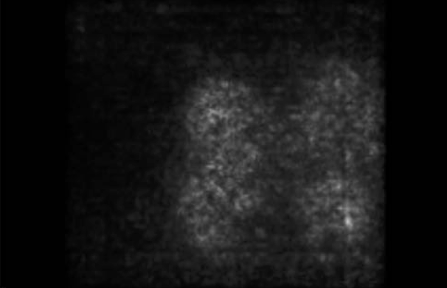
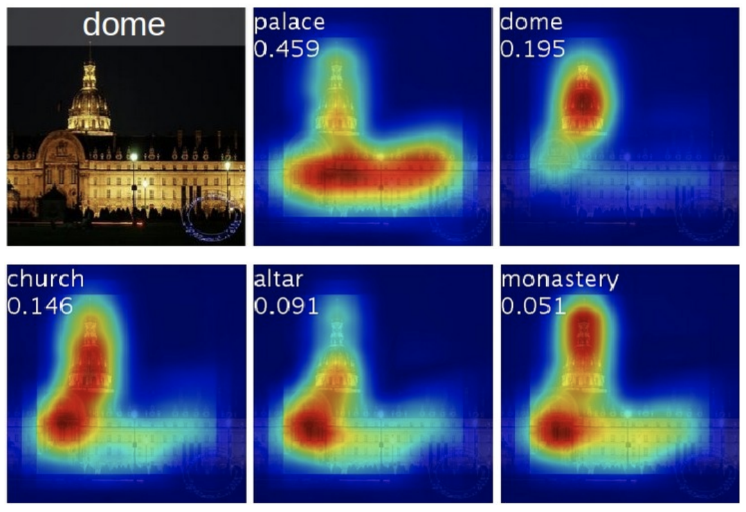
Class Activation Mapping (CAM)

$$F_k = \frac{1}{HW}\sum_{h,w} f_{h,w,k}$$
$$S_c = \sum_{k} w_{k,c} F_{k}$$
$$M_{c,h,w} = \sum_{k} w_{k,c} f_{h,w,k}$$
- Zhou et al, “Learning Deep Features for Discriminative Localization”, CVPR 2016
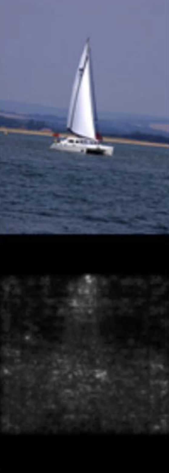
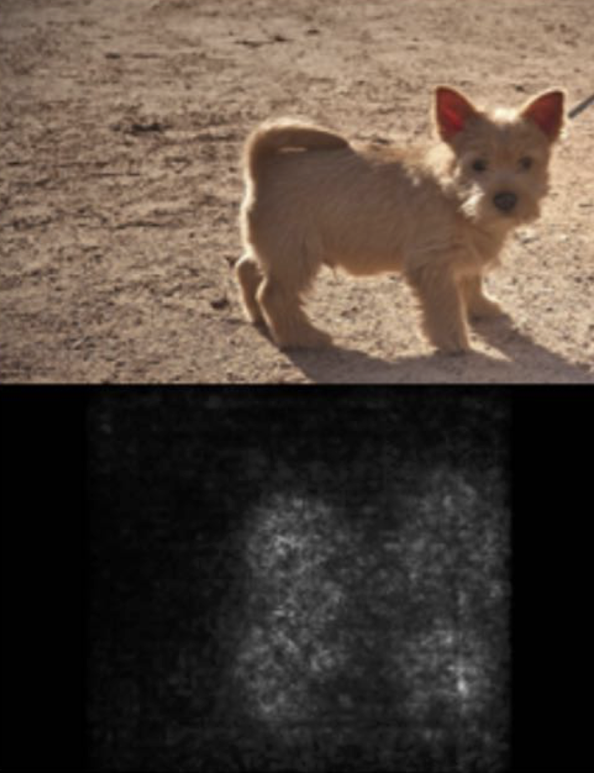
Class Activation Mapping Examples

Gradient Weighted Class Activation Mapping (Grad-CAM)
- Pick any layer, with activations $\mathbf{A} \in \mathbb{R}^{H\times W\times K}$
- Compute gradient of class score $\mathbf{S}_c$ with respect to $\mathbf{A}$ $$\frac{\partial \mathbf{S}_c}{\partial \mathbf{A}} \in \mathbb{R}^{H \times W \times K}$$
- Global average pool of the gradients to get weights $\alpha \in \mathbb{R}^K$: $$\alpha_k = \frac{1}{HW}\sum_{h,w} \frac{\partial \mathbf{S}_c}{\partial A_{h,w,k}}$$
- Compute activation map $\mathbf{M}^c \in \mathbb{R}^{H,W}$: $$M^c_{h,w} = ReLU(\sum_{k}\alpha_kA_{h,w,k})$$
- Selvaraju et al, "Grad-CAM: Visual Explanations from Deep Networks via Gradient-based Localization", CVPR 2017
Grad-CAM Examples

- Selvaraju et al, "Grad-CAM: Visual Explanations from Deep Networks via Gradient-based Localization", CVPR 2017
Grad-CAM Examples
- Can be applied to other tasks like image captioning, dense prediction etc.
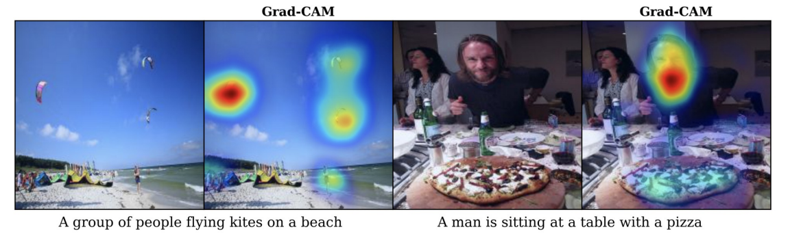
- Selvaraju et al, "Grad-CAM: Visual Explanations from Deep Networks via Gradient-based Localization", CVPR 2017
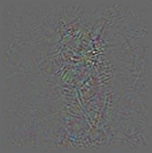
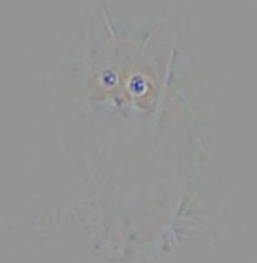
Visualizing CNN Features
Guided Backprop: Find part of the image a neuron responds to
Gradient Ascent: Generate a synthetic image that maximally activates a neuron
$$\mathbf{I}^* = \underset{\mathbf{I}}{\operatorname{arg max}} \color{cyan}{f(\mathbf{I})} + \color{yellow}{R(\mathbf{I})}$$
- $\color{cyan}{f(\mathbf{I})}$: Neuron Value
- $\color{yellow}{R(\mathbf{I})}$: Natural Image Regularizer
Gradient Ascent

$$\underset{\mathbf{I}}{\operatorname{arg max}} \color{cyan}{S_c(\mathbf{I})} -\lambda \|\mathbf{I}\|_2^2$$
- Initialize image to zeros
- Repeat:
- Forward image to compute current scores
- Backprop to get gradient of neuron value with respect to image pixels
- Make a small update to the image
Gradient Ascent
$$\underset{\mathbf{I}}{\operatorname{arg max}} S_c(\mathbf{I}) -\lambda\color{red}{\|\mathbf{I}\|_2^2}$$
- Simple Regularizer: Penalize $L_2$ norm of generated image
Gradient Ascent
$$\underset{\mathbf{I}}{\operatorname{arg max}} S_c(\mathbf{I}) -\lambda\|\mathbf{I}\|_2^2$$
- Better Regularizer: Penalize $L_2$ norm of image; also during optimization periodically
- Gaussian blur image
- Clip pixels with small values to 0
- Clip pixels with small gradients to 0
- Yosinski et.al. "Understanding Neural Networks through Deep Visualization" ICML DL Workshop 2014

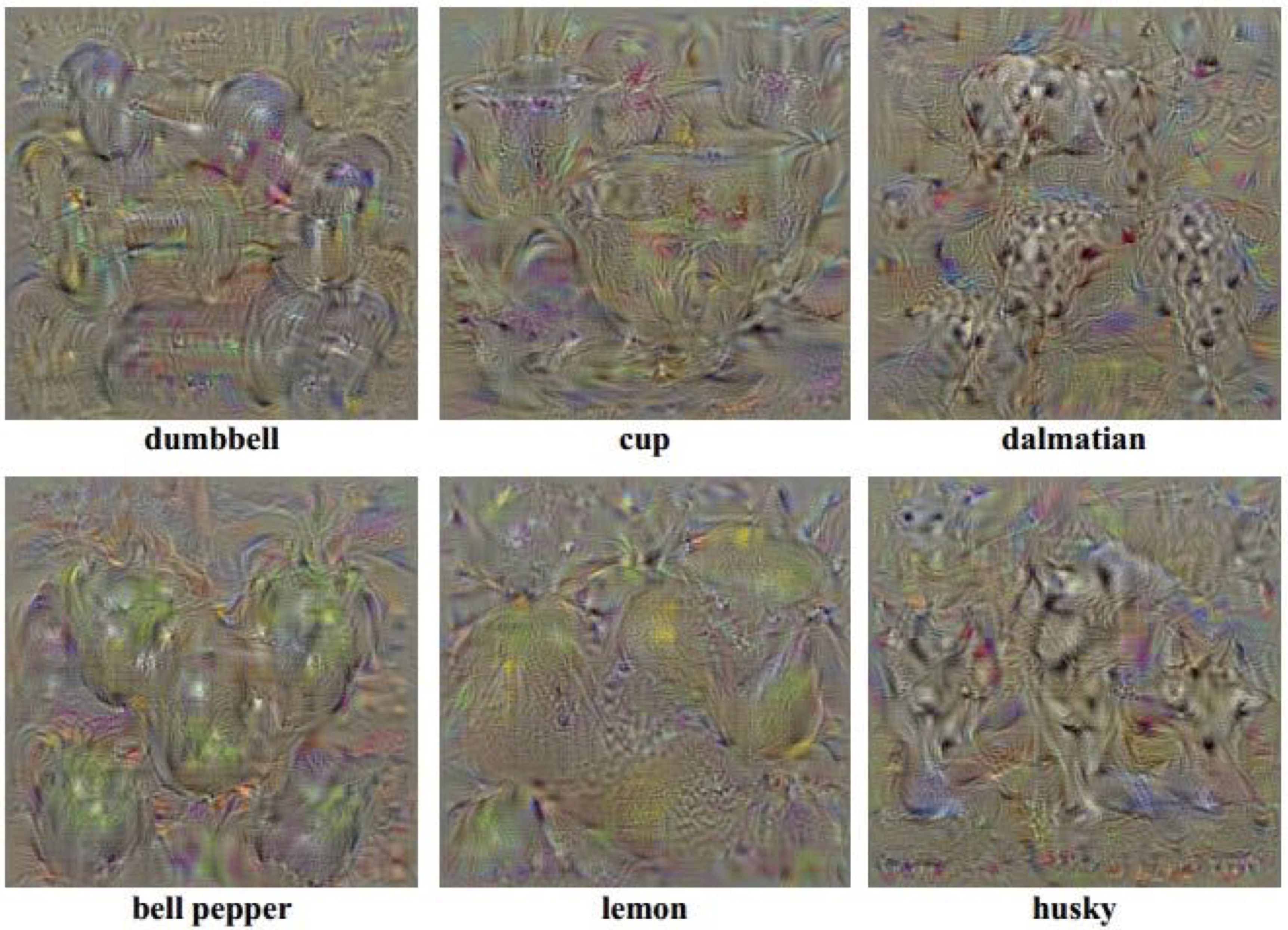
Gradient Ascent

Gradient Ascent
- Adding "multi-faceted" visualization gives even nicer results along with more careful regularization, center-bias.
- Nguyen et.al. "Multifaceted Feature Visualization: Uncovering the Different Types of Features Learned By Each Neuron in Deep Neural Networks" ICML Visualization for DL Workshop 2016
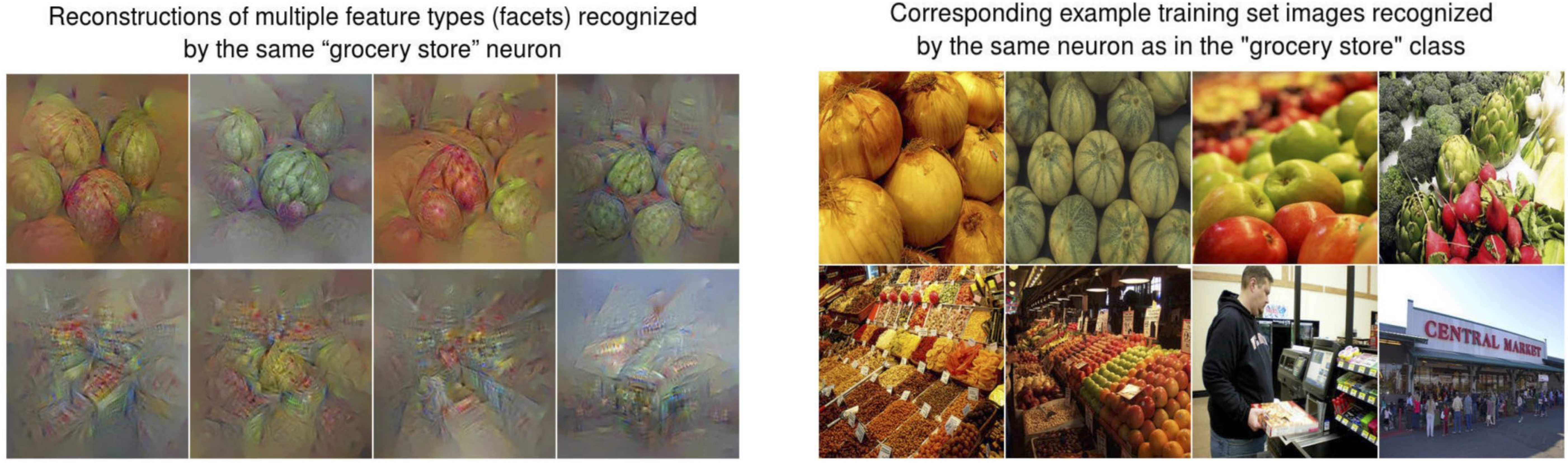
Gradient Ascent
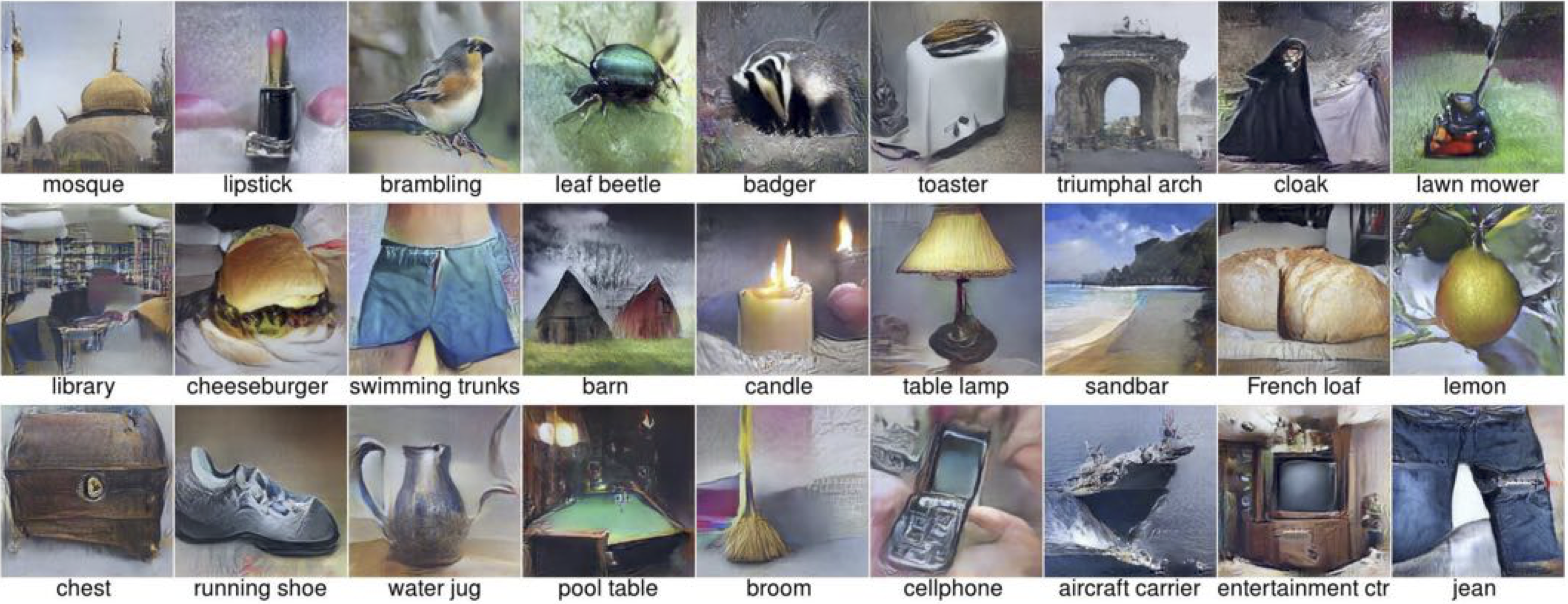
- Nguyen et.al. "Synthesizing the preferred inputs for neurons in neural networks via deep generator networks" NeurIPS 2016
Adversarial Examples
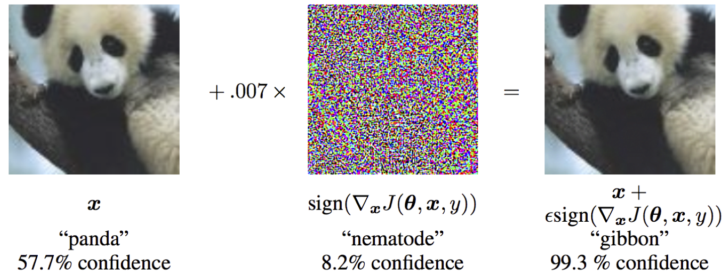
What are Adversarial Examples?
- One of the most surprising findings about neural nets has been the existence of adversarial inputs, i.e. inputs optimized to fool an algorithm.
- Given an image for one category (e.g. "cat"), compute the image gradient to maximize the network’s output unit for a different category (e.g. "dog")
- Perturb the image slightly in this direction, and chances are, the network will think it is a dog.
- A faster alternative is to take the sign of the entries in the gradient; this is called the fast gradient sign method.
Adversarial Examples: Recipe
- Start from an arbitrary image
- Pick an arbitrary category
- Modify image to maximize the class score (typically via SGD)
- Stop when the network is fooled
- Szegedy et.al. "Intriguing properties of neural networks" ICLR 2014
Adversarial Examples


Adversarial Examples
- 2013: this is cute
- The paper which introduced adversarial examples was titled "Intriguing Properties of Neural Networks."
- 2018: serious security threat
- No reliable methods yet to defend against them.
- 7 of 8 proposed defenses accepted to ICLR 2018 were cracked within days.
- Adversarial examples transfer to different networks trained on a totally separate training set!
- You don’t need access to the original network; you can train up a new network to match its predictions, and then construct adversarial examples for that.
- Attack carried out against proprietary classification networks accessed using prediction APIs (MetaMind, Amazon, Google)
Physical Attacks
Style Transfer
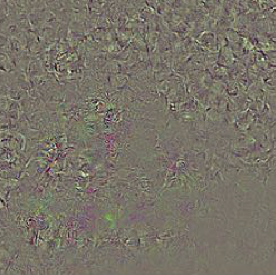
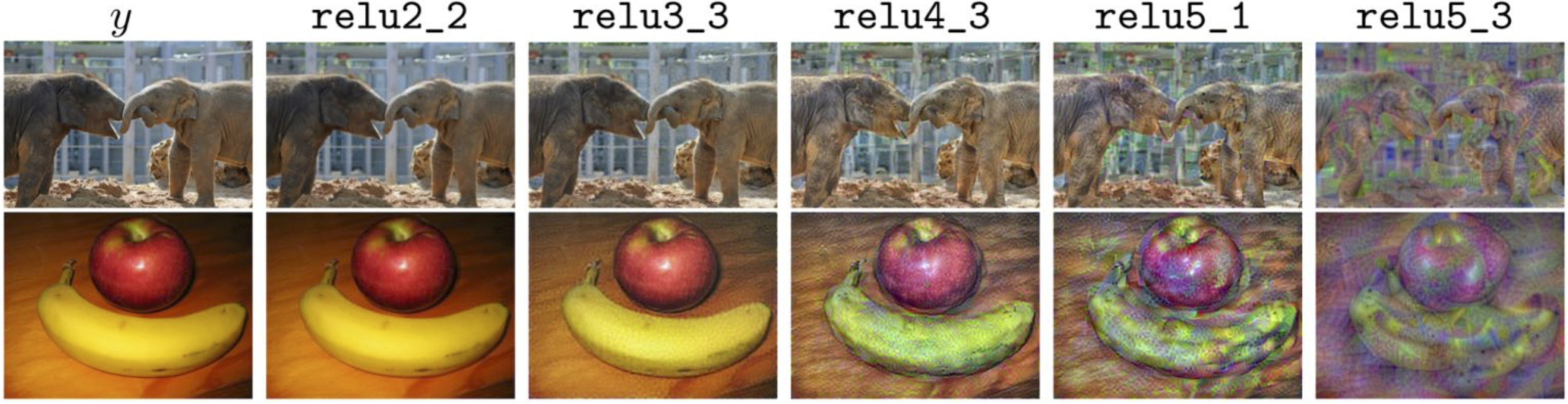
Feature Inversion
- Given a CNN activation for an image, find a new image that:
- Matches the given activation map
- "looks natural" (image prior regularization)
Feature Inversion
DeepDream: Feature Amplification
- Rather than synthesizing an image to maximize a specific neuron, instead try to amplify the neuron activations at some layer in the network
Equivalent to: $I^*=\underset{I}{\operatorname{arg max}} \sum_i f_i(I)^2$
- Choose an image and a layer in a CNN; repeat:
- Forward: compute activations at chosen layer
- Set gradient of chosen layer equal to its activation
- Backward: Compute gradient on image
- Update Image
What is Texture Synthesis
- Given a sample patch of some texture, can we generate a bigger image of the same texture?
- Generate pixels one at a time in scanline order;form neighborhood of already generated pixels and copy nearest neighbor from input.

Texture Synthesis: Nearest Neighbor

Texture Synthesis: Neural Networks

- Each layer of CNN gives $C \times H \times W$ tensor of features; $H \times W$ grid of $C$-dimensional vectors
- Outer product of two C-dimensional vectors gives $C \times C$ matrix of element wise products
- Average over all HW pairs gives Gram Matrix of shape $C \times C$ giving unnormalized covariance
- Efficient to compute; reshape features from $C\times H\times W$ to $\mathbf{F}=C\times HW$, the compute $\mathbf{G}=\mathbf{FF}^T$
Neural Texture Synthesis
- Pretrain a CNN on ImageNet (VGG-19)
- Run input texture forward through CNN, record activations on every layer; layer $i$ gives feature map of shape $C_i \times H_i \times W_i$
- At each layer compute the Gram matrix giving outer product of features: $G_{ij}^l = \sum_{k}F_{ik}^lF_{jk}^l$
- Initialize generated image from random noise
- Pass generated image through CNN, compute Gram matrix on each layer
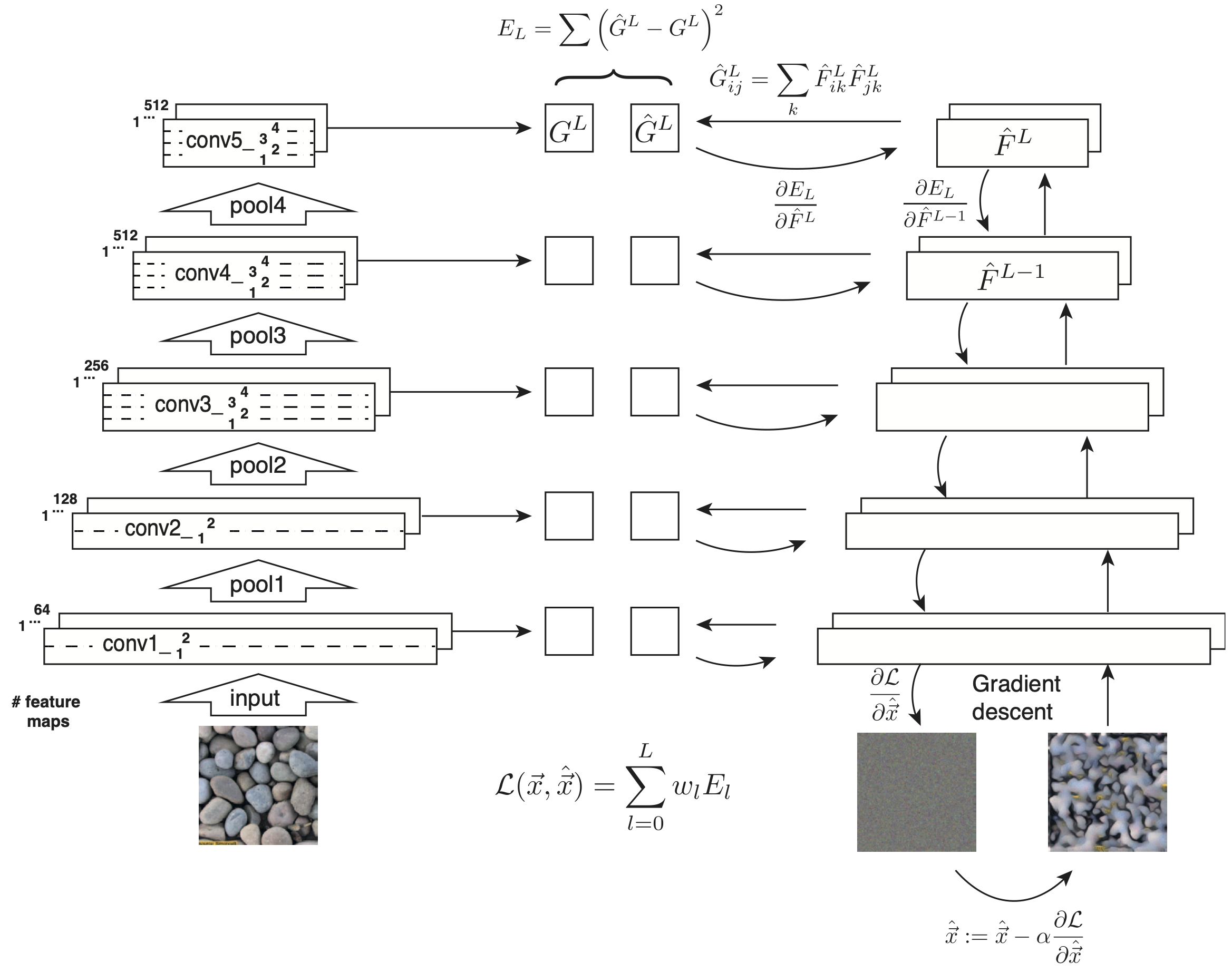
Neural Texture Synthesis
- Reconstructing texture from higher layers recovers larger features from the input texture

Neural Style Transfer
- Feature Reconstruction + Gram Reconstruction

Texture Synthesis (Gram Reconstruction)
Feature Reconstruction
- Johnson et al, "Perceptual Losses for Real-Time Style Transfer and Super-Resolution", ECCV 2016
Neural Style Transfer
- Gatys et al, "Image Style transfer using convolutional neural networks", CVPR 2016
Neural Style Transfer
Neural Style Transfer
Recall Normalization Methods?

Fast Neural Style Transfer
- Replacing Batch Normalization with Instance Normalization improves results.
- Ulyanov et al, "Texture Networks: Feed-forward Synthesis of Textures and Stylized Images", ICML 2016
- Ulyanov et al, "Instance Normalization: The Missing Ingredient for Fast Stylization", Arxiv 2016
One Network, Many Styles
- Dumoulin et al, "A Learned Representation for Artistic Style", ICLR 2017
One Network, Many Styles
- Use the same network for multiple styles using conditional instance normalization: learn separate scale and shift parameters per style
- Dumoulin et al, "A Learned Representation for Artistic Style", ICLR 2017
Summary
- Many methods for interpreting CNNs
- Activations: Nearest Neighbors, Dimensionality Reduction, Maximal Patches, Occlusion
- Gradients: Grad-CAM, Saliency Maps, Class Visualization, Adversarial Images, Feature Inversion
- Fun Applications: DeepDream, Style Transfer