Graph Neural Networks

Graph Neural Networks - II

CSE 849: Deep Learning

Vishnu Boddeti

Recap: Graph Structured Data

Standard CNN and RNN architectures don't work on this data.

Slide Credit: Xavier Bresson

Recap: Graph Definition

Graphs $\mathcal{G}$ are defined by:

Vertices $V$
Edges $E$
Adjacency matrix $\mathbf{A}$

Features:

Node features: $\mathbf{h}_i, \mathbf{h}_j$ (user type)
Edge features: $\mathbf{e}_{ij}$ (relation type)
Graph features: $\mathbf{g}$ (network type)

We want our main desiderata, permutation invariance and permutation equivariance, to still hold

Node Classification

Figure Credit: Jure Leskovec

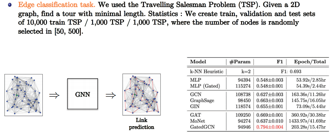
Link Prediction

Figure Credit: Jure Leskovec

Link Prediction: Social Networks

Figure Credit: Michael Bronstein

Link Prediction: Social Networks

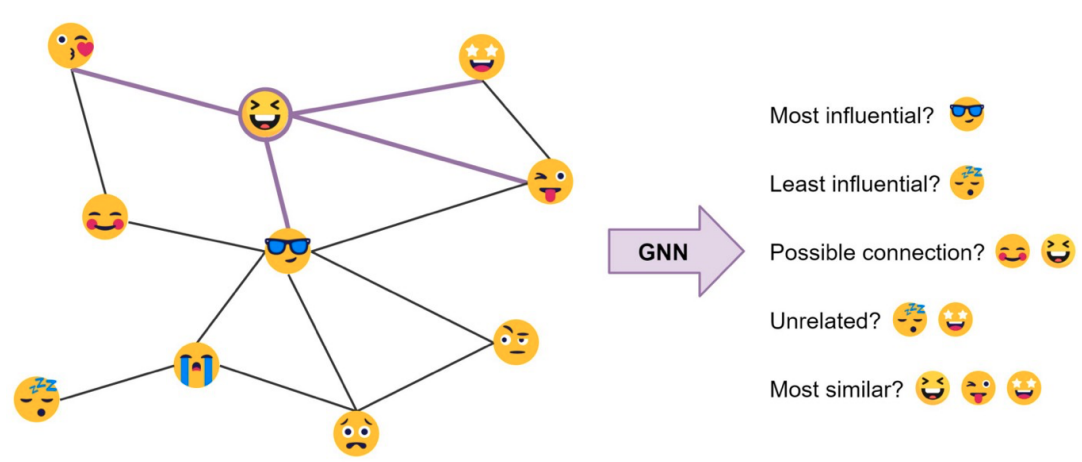
Figure Credit: Chaitanya Joshi

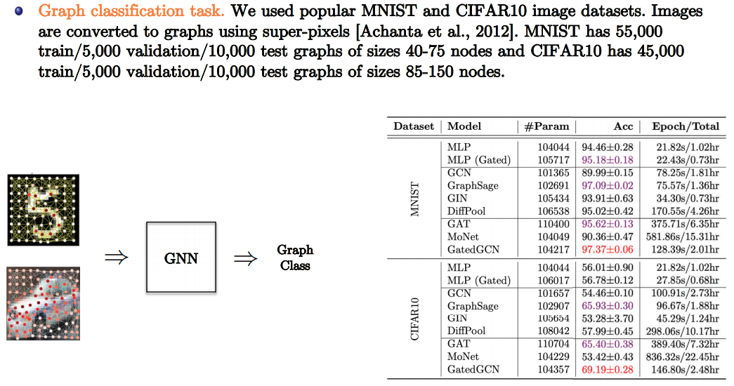
Graph Classification

Duvenaud et.al "Convolutional Networks on Graphs for Learning Molecular Fingerprints", NeurIPS 2015

How to construct GNN layers?

GNN Layers

We construct permutation-equivariant functions $f(\mathbf{X}, \mathbf{A})$ over graphs by shared application of a local permutation-invariant $g(\mathbf{x}_i, \mathbf{X}_{\mathcal{N}_i})$.

$f$: referred to as GNN layer
$g$: referred to as "diffusion", "propagation", "message passing"

How can we concretely define $g$:

many designs have been proposed
most proposed solutions fall into three spatial "flavors"

Three "Flavors" of GNN Layers

Convolutional $$\mathbf{h}_i=\phi\left(\mathbf{x}_i, \bigoplus_{j\in\mathcal{N}_i}c_{ij}\psi(\mathbf{x}_j)\right)$$

Attentional $$\mathbf{h}_i=\phi\left(\mathbf{x}_i, \bigoplus_{j\in\mathcal{N}_i}\alpha(\mathbf{x}_i,\mathbf{x}_j)\psi(\mathbf{x}_j)\right)$$

Message-Passing $$\mathbf{h}_i=\phi\left(\mathbf{x}_i, \bigoplus_{j\in\mathcal{N}_i}\psi(\mathbf{x}_i, \mathbf{x}_j)\right)$$

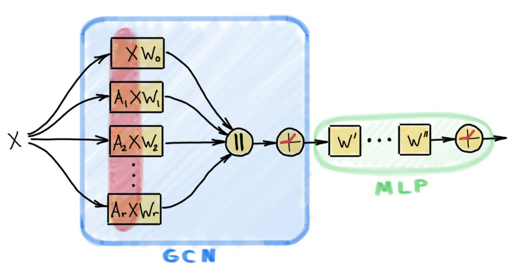
Convolutional GNN

Features of neighbours aggregated with fixed weights $c_{ij}$
The weights depend directly on $\mathbf{A}$

ChebyNet (Defferrard et al., NeurIPS 2016)
GCN (Kipf & Welling, ICLR 2017)
SGC (Wu et al., ICML 2019)

Useful for homophilous graphs and scaling up:

when edges encode label similarity

Attentional GNN

Features of neighbours aggregated with implicit weights via attention
Attention weights computed as $a_{ij}=a(\mathbf{x}_i,\mathbf{x}_j)$

MoNet (Monti et al., CVPR 2017)
GAT (Veličković, ICLR 2018)
GaAN (Zhang et al., UAI 2018)

Useful as "middle ground" w.r.t. capacity and scale:

Edges need not encode homophily
But still compute scalar value in each edge

Message-Passing GNN

Compute arbitrary vectors ("messages") to be sent across edges
Messages computed as $\mathbf{m}_{ij}=\psi(\mathbf{x}_i, \mathbf{x}_j)$

Interaction Networks (Battaglia et al., NeurIPS 2016)
MPNN (Gilmer, ICML 2017)
GraphNets (Battaglia et al., ICML 2018)

Most generic GNN layer:

May have scalability or learnability issues
Ideal for computational chemistry, reasoning and simulation

Node Embeddings

Learning Node Embedding

Early "successes" of deep learning on graphs was in embedding nodes into vectors $\mathbf{h}_u$ through an encoder.

At the time, was implemeted as look-up table

What makes a node representation good?

Graphs encode interesting structure.

node representations must preserve graph structure
Features of nodes $i$ and $j$ should be predictive of existence of edge $(i, j)$!

Can be implemented through an unsupervised loss.

$\mathbf{h}_i$ and $\mathbf{h}_j$ must be close iff $(i,j)\in\mathcal{E}$
can use standard cross-entropy loss $$\sum_{(i,j)\in\mathcal{E}}\log \sigma\left(\mathbf{h}_i^T\mathbf{h}_j\right) + \sum_{(i,j)\notin\mathcal{E}}\log\left(1-\sigma(\mathbf{h}_i^T\mathbf{h}_j)\right)$$

Random-Walks on Graphs

Link prediction objective is a special case of random-walk objectives

redefine the condition from $(i,j)\in\mathcal{E}$ to $i$ and $j$ co-occur in a (short) random-walk

Common unsupervised graph representation learning prior to GNNs

DeepWalk (Perozzi et al., KDD'14)
node2vec (Grover & Leskovec, KDD'16)
LINE (Tang et al., WWW'15)

Local Objectives vs Conv-GNNs

Random walk objectives inherently capture local similarities.
A (convolutional) GNN also summarises local information of the graph!

Neighbouring nodes tend to highly overlap in n-step neighbourhoods
Conv-GNN enforces similar features for neighbouring nodes by design.

DeepWalk-style models learn representations similar to that of convolutional GNN.
Corollary 1: Random-walk objectives can fail to provide useful signal to GNNs.
Corollary 2: At times, DeepWalk can be matched by an untrained Conv-GNN.

Deep Graph Informax (ICLR 2019)

Transformers vs GNNs

Transformers

Transformers is a special case of GCNs when the graph is fully connected.
The neighborhood $\mathcal{N}_i$ is the whole graph.

$$\begin{eqnarray} h_i^{l+1} &=& W^lConcat_{k=1}^K(\sum_{j\in\mathcal{N}_i}\alpha_{ij}^{k,l}V^{k,l}h_j^l) \\ \alpha_{ij}^{k,l} &=& Softmax_{\mathcal{N}_i}(\hat{\alpha}_{ij}^{k,l}) \\ \hat{\alpha}_{ij}^{k,l} &=& Q^{l,k}h_i^lK^{l,k}h_j^l \end{eqnarray}$$

Fully Connected Graph $$\begin{eqnarray} h_i^{l+1} &=& Concat_{k=1}^K(Softmax(Q^lK^{l^T})V^l)W^l \\ Q^l &=& h^lW^l_Q \\ K^l &=& h^lW^l_K \\ V^l &=& h^lW^l_V \\ \end{eqnarray}$$

Transformers

What does it mean to have a graph fully connected?

It becomes less useful to talk about graphs as each data point is connected to all other points. There is no particular graph structure that can be used.
It would be better to talk about sets rather than graphs in this case.
Transformers are Set Neural Networks.

They are today the best technique to analyze sets/bags of features.

Graph Transformers

Graph version of Transformer:

Attention mechanism in a one-hop neighborhood

Spectral GNNs

Convolution as Matrix Multiplication

Consider convolution over a sequence represented as cyclical grid graph:
Can we computed as a matrix multiplication with a circulant matrix s.t., $\mathbf{H}=\mathbf{CX}$

Circulant Matrices: Properties and Eignevectors

Circulant matrices commute

$\mathbf{C}(\mathbf{v})\mathbf{C}(\mathbf{w})=\mathbf{C}(\mathbf{w})\mathbf{C}(\mathbf{v})$ for any vectors $\mathbf{v}$ and $\mathbf{w}$

Matrices that commute are jointly diagonalisable.

eigenvectors are shared across all such matrices

Conveniently, the eigenvectors of circulants are the discrete Fourier basis: $$\phi_{l} = \frac{1}{\sqrt{n}}\left(1,e^{\frac{2\pi il}{n}},e^{\frac{4\pi il}{n}},\dots,e^{\frac{2\pi i(n-1)l}{n}}\right)^T \quad l=0,1,2,\dots,n-1$$
This can be easily computed by studying $\mathbf{C}([0, 1, 0, 0, 0, \dots])$, which is the shift matrix.

DFT and Convolution

We can eigendecompose any circulant matrix as $\mathbf{C}(\Lambda)=\Phi\Lambda\Phi^*$

$\Phi$ are the Fourier basis
diagonal values of $\Lambda$ are eignevalues

Convolution theorem naturally follows: $$f(\mathbf{X})=\mathbf{C}(\Lambda)\mathbf{X}=\Phi\Lambda\Phi^*\mathbf{X}=\Phi\begin{bmatrix}\hat{\lambda}_0 & & \\ & \ddots & \\ & & \hat{\lambda}_{n-1} \end{bmatrix}\Phi^*\mathbf{X}=\Phi(\hat{\lambda} \odot \hat{X})$$
If $\Phi$ is known, we can express convolution in terms of $\hat{\lambda}_i$ rather than spatial parameters $\mathbf{\theta}$.

Convolutions on Graphs

On graphs, convolutions of interest need to be more generic than circulants.

We can still use the concept of joint/common eigenbases.
If we know a "Fourier basis for graphs", $\Phi$, only focus on learning eigenvalues.

For grids, we wanted our convolutions to commute with shifts.

With adjacency matrix generalize to non-grids (shift matrix is special case for grid graph).
For convolution on regular grid of $n$ nodes, $\Phi$ was always the same (n-way DFT).
Now every graph will have its own $\Phi$.

Want our convolution to commute with A, but we cannot always eigendecompose A.
Instead, use the graph Laplacian matrix, $\mathbf{L} = \mathbf{D} - \mathbf{A}$, where $\mathbf{D}$ is the degree matrix.

Captures all adjacency properties in a mathematically convenient way.

Graph Laplacian

$$\mathbf{L}=\begin{bmatrix}2 & -1 & 0 & 0 & -1 & 0 \\-1 & 3 & -1 & 0 & -1 & 0 \\0 & -1 & 2 & -1 & 0 & 0 \\ 0 & 0 & -1 & 3 & -1 & -1 \\ -1 & -1 & 0 & -1 & 3 & 0 \\ 0 & 0 & 0 & -1 & 0 & 1\end{bmatrix}$$

Graph Fourier Transform

For undirected graphs, $\mathbf{L}$ is:

Symmetric
Positive semi-definite
easy to eigendecompose

We can express $\mathbf{L}=\Phi\Lambda\Phi^*$

Changing the eigenvalues in $\Lambda$ expresses any operation that commutes with $\mathbf{L}$.
Commonly referred to as the "graph Fourier transform" (Bruna et al., ICLR'14)

To convolve with a feature matrix $\mathbf{X}$, we do the following (learn $\lambda_i$): $$f(\mathbf{X})=\Phi\begin{bmatrix}\hat{\lambda}_0 & & \\ & \ddots & \\ & & \hat{\lambda}_{n-1} \end{bmatrix}\Phi^*\mathbf{X}$$

Spectral GNNs

Directly learning eigenvalues is typically inappropriate:

Not localized, doesn't generalize to other graphs, computationally expensive, etc.

Common solution: make eigenvalues $\mathbf{\Lambda}$ related to eigenvalues of $\mathbf{L}$

Typically by a degree-$k$ polynomial function, $p_k$
Yielding $f(x)=\mathbf{\Phi}p_k(L)\mathbf{\Phi^*x}$
Common variants:

Cubic splines (Bruna et al., ICLR'14)
Chebyshev polynomials (Defferrard et al., NeurIPS'16)
Cayley polynomials (Levie et al., Trans. Sig. Proc.'18)

Using a polynomial in $\mathbf{L}$ we can define a conv-GNN

With coefﬁcients defined by $c_{ij}= (p_k(L))_{ij}$

Transformers with Positional Encoding for Graphs

Transformers are typically defined on sets.
Order information can be provided to transformers through positional embeddings

Sines/cosines sampled depending on position $$\begin{equation} PE_{pos, 2i} = sin\left(\frac{pos}{10000^{\frac{2i}{d_{emb}}}}\right) \mbox{ and } PE_{pos, 2i+1} = cos\left(\frac{pos}{10000^{\frac{2i}{d_{emb}}}}\right) \end{equation}$$

Very similar to the DFT eigenvectors.
Positional embeddings can be interpreted as eigenvectors of the grid graph.
Same idea can be leveraged to define Transformers on Graphs

Just feed some eigenvectors of the graph Laplacian (columns of $\Phi$)
Graph Transformer from Dwivedi & Bresson (2021)

Probabilistic Graphical Models

Probabilistic Modeling

Treat graphs as probabilistic graphical models (PGMs)

Nodes: Random variables
Edges: dependencies between distributions

Encode independence and conditional independence

allows for compact representation of multivariate probabilistic distributions

$$p(a,b,c,d,e) = p(a)p(b)p(c|a,b)p(d|e)p(c|e)$$

Markov Random Fields

A particular PGM of interest is Markov Random Feild (MRF)

allows decompositio of joint distribution into product of edge potentials

MRFs are modelled through inputs $\mathbf{X}$ and latents $\mathbf{H}$.

latents are akin to node representations
inputs and latents for each node are are related to each other independently
latents are related accordingly to the edges of the graph

Joint probability distribution: $$p\left(\mathbf{X},\mathbf{H}\right)=\prod_{v\in\mathcal{V}}\phi\left(\mathbf{x}_v,\mathbf{h}_v\right)\prod_{(v_1,v_2)\in\mathcal{E}}\psi\left(\mathbf{h}_{v_1},\mathbf{h}_{v_2}\right)$$

$\phi(\cdot,\cdot)$ and $\psi(\cdot,\cdot)$ are real-valued potential functions

Mean-Field Inference

To embed nodes, we need to sample from the posterior, $p(\mathbf{H}|\mathbf{X})$

estimating the posterior is intractable, even if exact potential functions are known

One popular method of resolving this is mean-field variational inference

Assume posterior is approximated by a product of node-level densities $$p(\mathbf{H}|\mathbf{X})\approx \prod_{v \in \mathcal{V}}q(\mathbf{h}_v)$$
$q(\cdot)$ is a density that is easy to compute and sample from, e.g., Gaussian

$q(\cdot)$ can be estimated by minimizing $KL\left(\prod_{v}q(v|X)\|p(\mathbf{H}|\mathbf{X})\right)$ to true posterior
Minimising the KL is intractable, but it admits a favourable approximate algorithm

Mean-Field Inference as GNN

We can iteratively update $q(\cdot)$ starting from an initial guess $q^{(0)}(\mathbf{h})$ (variational inference): $$\log q^{(t+1)}(\mathbf{h}_i) = c_i + \log\phi(\mathbf{x}_i,\mathbf{h}_i) + \sum_{j\in\mathcal{N}_i}\int_{\mathbb{R}^k}q^t(\mathbf{h}_i)\log\psi(\mathbf{h}_i,\mathbf{h}_j)d\mathbf{h}_i$$
Aligns nicely with message-passing GNN. $$\mathbf{h}_i = \phi\left(\mathbf{x}_i,\bigoplus_{j\in\mathcal{N}_i}\psi(\mathbf{x}_i, \mathbf{x}_j)\right)$$

Graph Isomorphism Testing

How powerful are Graph Neural Networks?

GNNs are a powerful tool for processing real-world graph data

But they won't solve any task speciﬁed on a graph accurately!

Canonical example: deciding graph isomorphism

Can a GNN distinguish between two non-isomorphic graphs i.e., $\mathbf{h}_{G_1} \neq \mathbf{h}_{G_2}$?

Permutation invariance mandates that two isomorphic graphs will always be indistinguishable, so this case is OK.

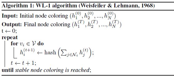
Weisfeiler-Leman Test

Simple but powerful way of distinguishing: pass random hashes of sums along the edges

Connection to conv-GNNs spotted very early; e.g., by GCN (Kipf & Welling, ICLR'17)

It explains why untrained GNNs work well!

Untrained $\sim$ random hash

The test can fail sometimes

GNNs are no more powerful than 1-WL

Over discrete features, GNNs can only be as powerful as the 1-WL test described before
One important condition for maximal power is an injective aggregator (e.g. sum)
Graph isomorphism network (GIN; Xu et al., ICLR'19) proposes a simple, maximally-expressive GNN, following this principle $$h_v^{(k)}=MLP^{(k)}\left(\left(1+\epsilon^{(k)}\right)\cdot h_v^{(k-1)}+\sum_{v \in \mathcal{N(v)}}h_v^{(k-1)}\right)$$

Higher-Order Graph Neural Networks

We can make GNNs stronger by analysing failure cases of 1-WL.
For example, just like 1-WL, GNNs cannot detect closed triangles

Augment nodes with randomised/positional features (Murphy et al., ICML'19 and You et al., ICML'19)
Can also literally count interesting subgraphs (Bouritsas et al., 2020)

k-WL labels subgraphs of k nodes together.

Exploited by 1-2-3-GNNs (Morris et al., AAAI'19)

If features are real-valued, injectivity of sum falls apart.

No aggregator is better than another aggregator.

Geometric Deep Learning

GNNs were described in terms of invariances and equivariances.
Many standard architectures like CNNs and Transformers can be recoverd by,

Local and equivariant layer speciﬁed over neighbourhoods
Activation functions
(Potentially: pooling layers that coarsen the structure)
Global and invariant layer over the entire domain

Can design a more general class of geometric deep learning architectures.

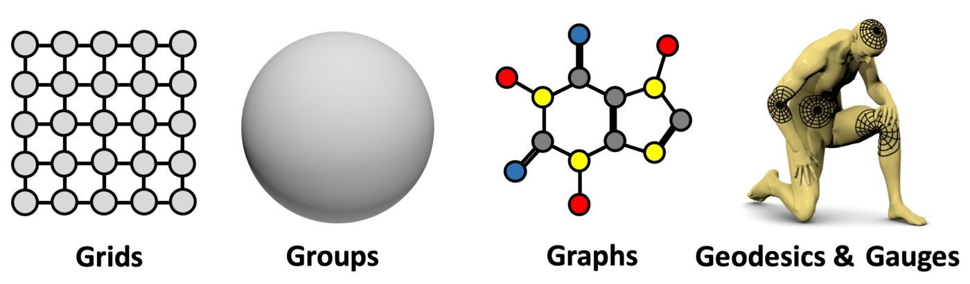
"Five Gs" of Geometric Deep Learning

Applications

Quantum Chemistry

Slide Credit: Xavier Bresson

Computer Vision

Slide Credit: Xavier Bresson

Combinatorial Optimization

Slide Credit: Xavier Bresson

Semi-Supervised Classification on Graphs

Setting:

Some nodes are labeled
All other nodes are unlabeled

Task:

Predict node label of unlabeled nodes

Evaluate loss on labeled nodes only:

$\mathcal{Y}_L$: set of labled node indices
$\mathbf{Y}$: label matrix
$\mathbf{Z}$: GCN output (after softmax)

Normalization and Depth

What kind of normalization can we do for graphs?

Node normalization
Pair normalization
Edge normalization

Does depth matter for GCNs?

Scalable Inception Graph Neural Networks

Figure Credit: Michael Bronstein

Scalable Inception Graph Neural Networks

Graph CNN Challenges

How to define compositionality on graphs (i.e. convolution, downsampling, and pooling on graphs)?
How to ensure generalizability across graphs?
And how to make them numerically fast? (as standard CNNs)
Scalability: millions of node, billions of edges
How to process dynamic graphs?
How to incorporate higher-order structures?
How powerful are graph neural networks?

limited theoretical understanding
message passing based GCN are no stronger than Weisfeiler-Lehman tests.

Getting Started

Lots of open questions and uncharted territory.
Standardized Benchmarks: Open Graph Benchmark
Software Packages: Pytorch Geometric or Deep Graph Library

Recap: Graph Structured Data

Recap: Graph Definition

Node Classification

Link Prediction

Link Prediction: Social Networks

Link Prediction: Social Networks

Graph Classification

How to construct GNN layers?

GNN Layers

Three "Flavors" of GNN Layers

Convolutional GNN

Attentional GNN

Message-Passing GNN

Node Embeddings

Learning Node Embedding

What makes a node representation good?

Random-Walks on Graphs

Local Objectives vs Conv-GNNs

Transformers vs GNNs

Transformers

Transformers

Graph Transformers

Spectral GNNs

Convolution as Matrix Multiplication

Circulant Matrices: Properties and Eignevectors

DFT and Convolution

Convolutions on Graphs

Graph Laplacian

Graph Fourier Transform

Spectral GNNs

Transformers with Positional Encoding for Graphs

Probabilistic Graphical Models

Probabilistic Modeling

Markov Random Fields

Mean-Field Inference

Mean-Field Inference as GNN

Graph Isomorphism Testing

How powerful are Graph Neural Networks?

Weisfeiler-Leman Test

GNNs are no more powerful than 1-WL

Higher-Order Graph Neural Networks

Geometric Deep Learning

Geometric Deep Learning

"Five Gs" of Geometric Deep Learning

Applications

Quantum Chemistry

Computer Vision

Combinatorial Optimization

Semi-Supervised Classification on Graphs

Normalization and Depth

Scalable Inception Graph Neural Networks

Scalable Inception Graph Neural Networks

Graph CNN Challenges

Getting Started

ICLR 2021 Talk on GNNs