Generative Models - Introduction
CSE 849: Deep Learning
Generative Models
- Unsupervised Learning: only use the inputs $\mathbf{x}^{(t)}$ for learning.
- automatically extract meaningful features for your data
- leverage the availability of unlabeled data
- add a data-dependent regularizer to training
- Many neural network based unsupervised learning approaches exist
- Autoregressive Models
- Autoencoders (Variational Autoencoders)
- Generative Adversarial Networks
- Flow Models
- Diffusion Models
Why Generative Models?
- Move beyond associating inputs to outputs
- Recognize objects in the world and their factors of variation
- Understand and imagine how the world evolves
- Detect surprising events in the world
- Imagine and generate rich plans for the future
- Establish concepts as useful for reasoning and decision making
Desiderata
- We want to estimate distributions of complex, high-dimensional data
- A $128\times 128\times 3$ image lies in a ~50,000-dimensional space
- We also want computational and statistical efficiency
- Efficient training and model representation
- Expressiveness and generalization
- Sampling quality and speed
- Compression rate and speed
Simplest Generative Model
Learning Through Histograms
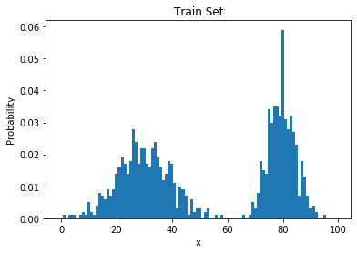
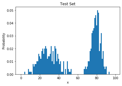
- Our goal: estimate $p_{data}$ from samples $x^{(1)}, \dots, x^{(n)} \sim p_{data}(x)$
- Suppose the samples take on values in a finite set $\{1, \dots, k\}$
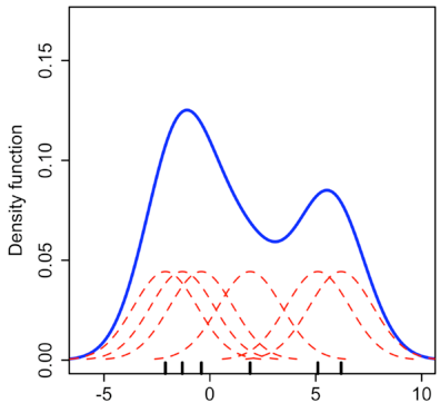
- The model: a histogram
- (Redundantly) described by k nonnegative numbers: $p_1, \dots, p_k$
- To train this model: count frequencies $$\begin{equation} p_i = \frac{\mbox{# times i appears in the dataset}}{\mbox{# points in the dataset}} \end{equation}$$
Inference and Sampling
- Inference (querying $p_i$ for arbitrary $i$): simply a lookup into the array $p_1, \dots, p_k$
- Sampling (lookup into the inverse cumulative distribution function)
- From the model probabilities $p_1, \dots, p_k$, compute the cumulative distribution
- Draw a uniform random number $u \sim [0, 1]$
- Return the smallest $i$ such that $u \leq F_i$
- Are we done?
Failure in High Dimensions
- No, because of the curse of dimensionality. Counting fails when there are too many bins.
- (Binary) MNIST: 28x28 images, each pixel in {0, 1}
- There are $2^{784} \approx 10^{236}$ probabilities to estimate
- Any reasonable training set covers only a tiny fraction of this
- Each image influences only one parameter. No generalization whatsoever!
Poor Generalization
- learned histogram = training data distribution
- poor generalization
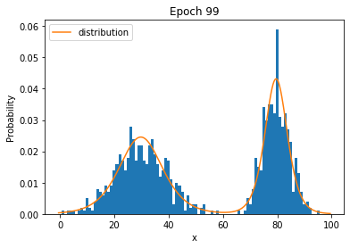
Parameterized Distributions
Status
- Issues with Histograms
- High dimensions: won't work
- Even 1-d: if many values in the domain, prone to overfitting
- Solution: function approximation. Instead of storing each probability, store a parameterized function $p_{\mathbf{\theta}}(\mathbf{x})$
Applications
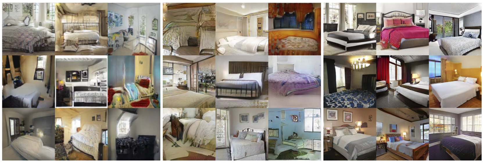
Applications: Data Generation
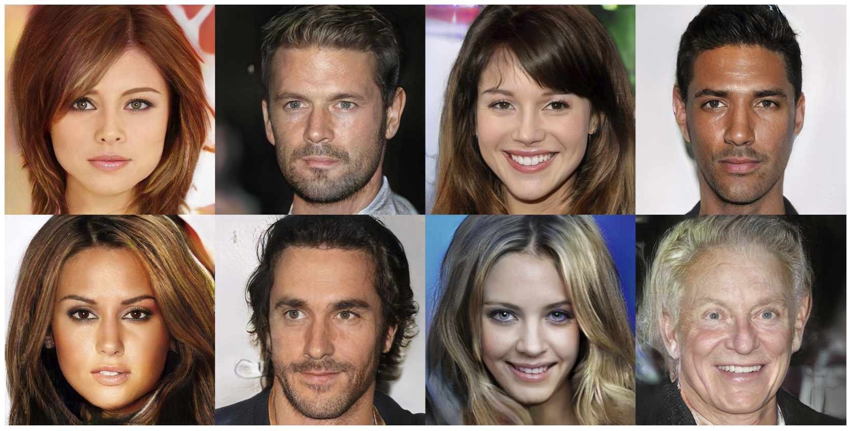
Applications: Data Generation
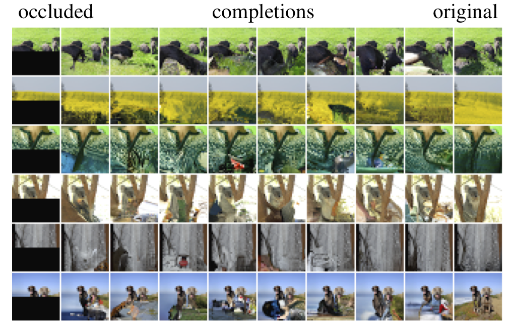
Applications: Data Imputation, Denoising, In-painting
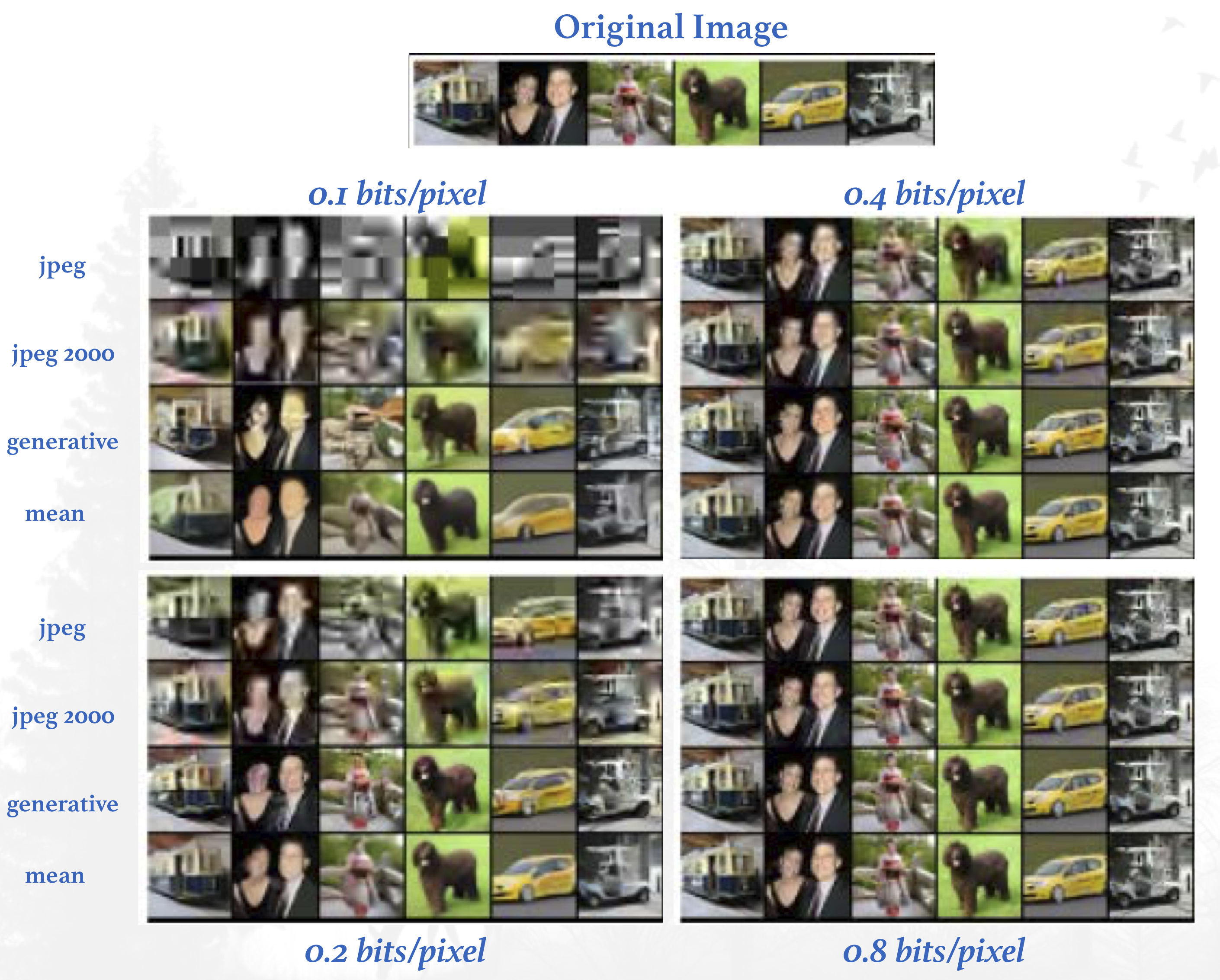
Applications: Communication and Compression
Learning Generative Models
Likelihood-based generative models
- Our goal: estimate $p_{data}$ from samples $x^{(1)}, \dots, x^{(n)} \sim p_{data}(x)$
- Now we introduce function approximation: learn $\mathbf{\theta}$ so that $p_{\mathbf{\theta}}(x) \approx p_{data}(x)$
- How do we design function approximators to effectively represent complex joint distributions over $\mathbf{x}$, yet remain easy to train?
- There will be many choices for model design, each with different trade-offs and different compatibility criteria.
- Designing the model and the training procedure go hand-in-hand.
Fitting Distributions
- Given data $x^{(1)}, \dots, x^{(n)}$ sampled from a "true" distribution $p_{data}$
- Set up a model class: a set of parameterized distributions $p_{\mathbf{\theta}}$
- Pose a search problem over parameters $$\begin{equation} \underset{\mathbf{\theta}}{\operatorname{arg min}} loss(\mathbf{\theta},\mathbf{x}^{(1)}, \dots, \mathbf{x}^{(n)}) \end{equation}$$
- Want the loss function + search procedure to:
- Work with large datasets ($n$ is large, say millions of training examples)
- Yield $\mathbf{\theta}$ such that $p_{\mathbf{\theta}}$ matches $p_{data}$ - i.e. the training algorithm works. Think of the loss as a distance between distributions.
- Note that the training procedure can only see the empirical data distribution, not the true data distribution: we want the model to generalize.
Maximum Likelihood
- Maximum likelihood: given a dataset $x^{(1)}, \dots, x^{(n)}$, find $\mathbf{\theta}$ by solving the optimization problem $$\begin{equation} \underset{\mathbf{\theta}}{\operatorname{arg min}} loss(\mathbf{\theta},\mathbf{x}^{(1)}, \dots, \mathbf{x}^{(n)}) = \frac{1}{n}\sum_{i=1}^n -\log p_{\mathbf{\theta}}(\mathbf{x}^{(i)}) \end{equation}$$
- Statistics tells us that if the model family is expressive enough and if enough data is given, then solving the maximum likelihood problem will yield parameters that generate the data
- Equivalent to minimizing KL divergence between the empirical data distribution and the model $$\begin{eqnarray} \hat{p}_{data}(\mathbf{x}) &=& \frac{1}{n}\sum_{i=1}^n\mathbf{1}[\mathbf{x}==\mathbf{x}^{(i)}] \\ KL(\hat{p}_{data}||p_{\mathbf{\theta}}) &=& \mathbb{E}_{\mathbf{x}\sim\hat{p}_{data}}[-\log p_{\mathbf{\theta}}(\mathbf{x})] - H(\hat{p}_{data}) \end{eqnarray}$$
Stochastic Gradient Descent
- Maximum likelihood is an optimization problem. How do we solve it?
- Stochastic gradient descent (SGD).
- SGD minimizes expectations: for a differentiable function of $\theta$, it solves $$\begin{equation} \underset{\mathbf{\theta}}{\operatorname{arg min}} \mathbb{E}[f(\mathbf{\theta})] \end{equation}$$
- With maximum likelihood, the optimization problem is $$\begin{equation} \underset{\mathbf{\theta}}{\operatorname{arg min}} \mathbb{E}_{\mathbf{x}\sim\hat{p}_{data}}[-\log p_{\mathbf{\theta}}(\mathbf{x})] \end{equation}$$
- Why maximum likelihood + SGD? It works with large datasets and is compatible with neural networks.
Designing The Model
- Key requirement for maximum likelihood + SGD: efficiently compute $\log p(x)$ and its gradient
- We will choose models $p_{\mathbf{\theta}}$ to be deep neural networks, which work in the regime of high expressiveness and efficient computation (assuming specialized hardware)
- How exactly do we design these networks?
- Any setting of $\mathbf{\theta}$ must define a valid probability distribution over $\mathbf{x}$: $$\begin{equation} \mbox{for all } \mathbf{\theta}, \mbox{ } \sum_{\mathbf{x}}p_{\mathbf{\theta}}(\mathbf{x}) = 1 \mbox{ and } p_{\mathbf{\theta}}(\mathbf{x})\geq 0 \mbox{ for all } \mathbf{x} \end{equation}$$
- $\log p_{\mathbf{\theta}}(\mathbf{x})$ should be easy to evaluate and differentiate with respect to $\mathbf{\theta}$
- This can be tricky to set up!
Simple Generative Models
Example: Autoencoder
- Autoencoders consists of:
- encoder
- decoder
- Encoder and decoder are trained to reproduce its input at the output layer.


- Encoder: \begin{eqnarray} h(\mathbf{x}) &=& g(\mathbf{a}(\mathbf{x})) \nonumber \\ &=& sigmoid(\mathbf{b}+\mathbf{W}\mathbf{x}) \nonumber \end{eqnarray}
- Decoder: \begin{eqnarray} \hat{\mathbf{x}} &=& o(\hat{\mathbf{a}}(\mathbf{x})) \nonumber \\ &=& sigmoid(\mathbf{c}+\mathbf{W}^{\ast}h(\mathbf{x})) \nonumber \end{eqnarray}
Loss Function
- Binary Inputs
- cross-entropy \begin{equation} L = -\sum_{k} x_k\log(\hat{x}_k) + (1-x_k)\log(1-\hat{x}_k) \nonumber \end{equation}
- Real-Valued Inputs
- sum-of-squared differences
- we use a linear activation function at the output \begin{equation} L = \frac{1}{2}\sum_{k}(x_k-\hat{x}_k)^2 \nonumber \end{equation}
- Gradient: $\nabla_{\mathbf{\hat{a}}(\mathbf{x}^{t})}L = \mathbf{\hat{x}}^{t} - \mathbf{x}^{t}$
- when weights are tied, $\nabla_{\mathbf{W}}L$ is the sum of two gradients.
Under-complete Hidden Layers
- Hidden layer is under-complete if smaller than the input layer
- hidden layer "compresses" the input
- will compress well only for the training distribution
- Hidden units will be
- good features for the training distribution
- but bad for other types of input

- Training Distribution:
- Other Distribution:


Over-complete Hidden Layer
- Hidden layer is over-complete if greater than the input layer
- no compression in hidden layer
- each hidden unit could copy a different input component
- No guarantee that the hidden units will extract meaningful structure.

Denoising Autoencoder
- Representation should be robust to introduction of noise.
- randomly assign subset of inputs to 0, with probability $\nu$
- Gaussian additive noise
- reconstruction $\hat{\mathbf{x}}$ computed from the corrupted input $\tilde{\mathbf{x}}$.
- Loss function compares $\hat{\mathbf{x}}$ reconstruction with the noiseless input $\mathbf{x}$.

Linear Autoencoder
- Given a linear decoder, what is the best encoder for MSE loss?
- Theorem:
- let $\mathbf{A}$ be any matrix, with SVD $\mathbf{A}=\mathbf{U\Sigma V}^T$
- Decomposition of rank $K$: $\mathbf{U}_{.,\leq K}\Sigma_{\leq K, \leq K}\mathbf{V}^T_{.,\leq K}$
- then, the matrix $\mathbf{B}$ of rank $K$ that is closest to $\mathbf{A}$: \[\mathbf{B}^{*} = \underset{\mathbf{B} \mbox{ s.t. rank}(\mathbf{B})=K}{\operatorname{arg min}} \|A-B\|_{F}\] is $\mathbf{B}^{*}=\mathbf{U}_{.,\leq K}\Sigma_{\leq K, \leq K}\mathbf{V}^T_{.,\leq K}$
- If inputs are normalized as follows: $\mathbf{x}^t = \frac{1}{\sqrt{T}}\left(\mathbf{x}^t-\frac{1}{T}\sum_{t'=1}^T\mathbf{x}^{t'}\right)$
- encoder corresponds to Principal Component Analysis (PCA)
- singular values and (left) vectors = the eigenvalues/eigenvectors of covariance matrix
What you will learn
- $p_{\mathbf{\theta}}(\mathbf{x})$ Use deep networks as function approximators.
- fully connected
- convolutional networks
- recurrent networks
- Machinery
- Design of probabilistic models
- Memoryless and Amortized Inference
- Stochastic Optimization
- Underlying goal: Density Estimation
A Probabilistic Viewpoint
- Goal: modeling $p_{data}$


