Score Matching and Diffusion Models - I

CSE 849: Deep Learning

Vishnu Boddeti

A Probabilistic Viewpoint

• Goal: modeling $p_{data}$

Fully Observed Models

Transformation Models (likelihood free)

Latent Variable Models (observation noise)

Undirected Latent Variable Models (hidden factors)

Core Idea

• Interpolating between two distributions:


• Density:




• Samples:

Core Idea

• Interpolating between two distributions:
• The data distribution is denoted $p_{data} \in \mathcal{P}(\mathbb{R}_d)$.
• The easy-to-sample distribution is denoted $p_{ref} \in \mathcal{P}(\mathbb{R}_d)$.
• $p_{ref}$ is usually the standard multivariate Gaussian.
• Going from the data to the easy-to-sample distribution: noising process.
• Going from the easy-to-sample to the data distribution: generative process.
• How to invert the forward noising process?

Ancestral Sampling: Forward

• Let $N \in \mathbb{N}$ with $N > 0$ and consider $p$ a density on $(\mathbb{R}^d)^{N+1}$ such that for any $\mathbf{x}_{0:N} = {\mathbf{x}_k}_{k=0}^N$ we have $$p(\mathbf{x}_{0:N}) = p_0(\mathbf{x}_0)\prod_{i=1}^N p_{k+1|k}(\mathbf{x}_{k+1}|\mathbf{x}_k)$$
• This the forward decomposition of $p$.

Ancestral Sampling: Backward

• For any $k \in \{0,\dots,N-1\}$ we define the marginal $p_{k+1}$ for any $\mathbf{x}_{k+1}\in \mathbb{R}^d$. $$p_{k+1}(\mathbf{x}_{k+1}) = \int_{\mathbb{R}^d} p_k(\mathbf{x}_k)p_{k+1|k}(\mathbf{x}_{k+1}|\mathbf{x}_k)d\mathbf{x}_k$$
• Assume that for any $k \in \{0,\dots,N\}, p_k > 0$ and define $p_{k|k+1}$ for any $\mathbf{x}_k, \mathbf{x}_{k+1} \in \mathbb{R}^d$ $$p_{k|k+1}(\mathbf{x}_k|\mathbf{x}_{k+1})=\frac{p_{k+1|k}(\mathbf{x}_{k+1}|\mathbf{x}_k)p_{k}(\mathbf{x}_{k})}{p_{k+1}(\mathbf{x}_{k+1})}$$
• We obtain the backward decomposition $$p(\mathbf{x}_{0:N}) = p_N(\mathbf{x}_N)\prod_{i=0}^{N-1} p_{k|k+1}(\mathbf{x}_{k}|\mathbf{x}_{k+1})$$

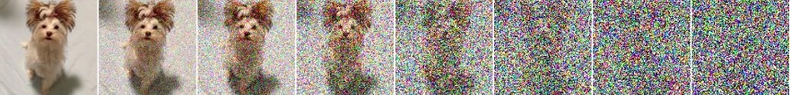
Adding noise to images

• We are given an input dataset $$\mathcal{D} = \{x_i\}_{i=1}^N \subset \mathbb{R}^d$$
• We assume that these images are independent samples of a common distribution $p_0$ over $\mathbb{R}^d$.
• Consider the random process that consists of adding noise to images: $$\mathbf{x}_t = \mathbf{x}_0 + \mathbf{w}_t, \quad t \in [0,T]$$ where $\mathbf{x}_0 \sim p_0$ is a sample image and $\mathbf{w}_t$ is a Brownian motion (also called Wiener process).

Brownian Motion

• Real-valued: A standard (real-valued) Brownian motion (also called Wiener process is a stochastic process $(w_t)_{t \geq 0}$ such that
• $w_0=0$
• With probability one, the function $t \mapsto w_t$ is continuous.
• The process $(w_t)_{t \geq 0}$ has stationary, independent increment.
• $w_t \sim \mathcal{N}(0,t)$
• Direct consequences:
• For $s < t$, $w_s$ and $w_t-w_s$ are independent and $w_{t-s} \sim \mathcal{N}(0, t-s)$
• Markovian random field.
• $\mathbb{R}^d$-valued: A standard $\mathbb{R}^d$-valued Brownian motion $(\mathbf{w}_t)_{t \geq 0}$ is made of $d$ independent real-valued Brownian motion $$ \mathbf{w}_t = (w_{t,1}, \cdots, w_{t,d}) \in \mathbb{R}^d $$

Adding noise to images

• Adding noise to images: $\mathbf{x}_t = \mathbf{x}_0 + \mathbf{w}_t, t\in[0,T].$
• This corresponds to the stochastic differential equation (SDE): $$d\mathbf{x}_t = d\mathbf{w}_t, \text{ with initial condition } \mathbf{x}_0 \sim p_0.$$
• We denote by $p_t$ the distribution of $\mathbf{x}_t$ at time $t \in [0, T]$. What is $p_t$? $$p_t = p_0 \ast \mathcal{N}(\mathbf{0}, t\mathbf{I}_d)$$
• This corresponds to applying the heat equation starting from $p_0$: $$\partial_tp_t(\mathbf{x})=\frac{1}{2}\nabla^2_xp_t(\mathbf{x}_t) \text{ with } p_{t=0}=p_0$$
• This PDE is called the Fokker-Planck equation associated with the SDE.
• This is an example of diffusion equation.

Diffusion SDE and Fokker-Planck equation

• More generally we will consider diffusion SDE of the form (Song et al., 2021b): $$d\mathbf{x}_t = \mathbf{f}(\mathbf{x}_t, t)dt + g(t)d\mathbf{w}_t$$
• $\mathbf{f}:\mathbb{R}^d\times[0,T]\rightarrow \mathbb{R}^d$ is called the drift. External deterministic force that drives $\mathbf{x}_t$ in the direction of $\mathbf{f}(\mathbf{x}_t, t)$
• $g:[0,T]\rightarrow [0,+\infty)$ is the diffusion coefficient
• The corresponding Fokker-Planck equation is: $$ \partial_tp_t(\mathbf{x})= - \nabla_{\mathbf{x}}(\mathbf{f}(\mathbf{x}_t,t)p_t(\mathbf{x})) + \frac{1}{2}g(t)^2\nabla^2_{\mathbf{x}}p_t(\mathbf{x})$$

Diffusion SDE: Two examples

• Ornstein-Uhlenbeck process: $$d\mathbf{x}_t = -\mathbf{x}_t dt + \sqrt{2}d\mathbf{w}_t$$
• Geometric Brownian motion: $$d\mathbf{x}_t = \mathbf{x}_t dt + \mathbf{x}_t d\mathbf{w}_t$$

Diffusion SDE: Two examples

• Example 1: Variance exploding diffusion (VE-SDE) $$ \begin{aligned} \text{SDE:} & \quad d\mathbf{x}_t = d\mathbf{w}_t \\ \text{Solution:} & \quad \mathbf{x}_t = \mathbf{x}_0 + \mathbf{w}_t \\ \text{Variance:} & \quad Var(\mathbf{x}_t) = Var(\mathbf{x}_0) + t \end{aligned} $$
• Example 2: Variance preserving diffusion (VP-SDE) $$ \begin{aligned} \text{SDE:} & \quad \mathbf{x}_t = -\beta_t\mathbf{x}_tdt + \sqrt{2\beta_t}d\mathbf{w}_t \\ \text{Solution:} & \quad \mathbf{x}_t = e^{-B_t}\mathbf{x}_0 + \int_{0}^te^{B_2-B_t}\sqrt{2\beta_s}d\mathbf{w}_s \text{ with } B_t=\int_{0}^t\beta_tdt \\ \text{Variance:} & \quad Var(\mathbf{x}_t) = e^{-2B_t}Var(\mathbf{x}_0) + 1 - e^{-2B_t} \end{aligned} $$
• Both variants have the form $\mathbf{x}_t = \alpha_t \mathbf{x}_0 + \beta_t \mathbf{Z}_t: \mathbf{x}_t$ is a rescaled noisy version of $\mathbf{x}_0$ and the noise is more and more predominant as time grows.

Diffusion SDE: Forward

Numerical scheme for diffusion SDE

• In general we do not have a close form formula for $\mathbf{x}_t$.
• Diffusion SDEs can be approximately simulated using numerical schemes such as the Euler-Maruyama scheme:
• Using the time step $h = T/N$ with $N + 1$ times $t_n=nh, n \in {0, \dots, N}$, define $\mathbf{X}_0 = \mathbf{x}_0$ and $$\mathbf{X}_{n+1} = \mathbf{X}_n + h\mathbf{f}(\mathbf{X}_n, t_n) + g(t_n)(\mathbf{w}_{t_{n+1}}-\mathbf{w}_{t_n}), n=\{1,\dots,N-1\}.$$
• Remark that $\mathbf{w}_{t_{n+1}}- \mathbf{w}_{t_n} \sim \mathcal{N}(\mathbf{0}, h\mathbf{I}_d)$ and is independent of $\mathbf{X}_n$: $$\mathbf{X}_{n+1} = \mathbf{X}_n + h\mathbf{f}(\mathbf{X}_n, t_n) + \sqrt{h}g(t_n)\mathbf{Z}_n, \text{ with } \mathbf{Z}_n\sim\mathcal{N}(\mathbf{0}, \mathbf{I}_d), n=\{1,\dots,N-1\}.$$

Reversed Diffusion

• For diffusion SDEs, as $t$ grows $p_t$ is closer and closer to a normal distribution.
• We will consider that at the final time $t=T$ large enough so that $p_T$ can be considered to be a normal distribution.
• For generative modeling, we want to reverse the process:
• Start by generating $\mathbf{x}_T \sim p_T \approx \mathcal{N}(\mathbf{0}, \sigma_T^2 \mathbf{I}_d)$.
• Simulate $(\mathbf{x}_{T-t}) t \in [0,T]$ such that $\mathbf{x}_{T-t} \sim p_{T-t}$.

Reversed Diffusion Continued...

• Reversed diffusion: What is the SDE satisfied by $\mathbf{x}_{T-t}$? $$ d\mathbf{x}_t = \mathbf{f}(\mathbf{x}_t, t)dt + g(t)d\mathbf{w}_t$$
• has the associated Fokker-Planck equation $$ \partial_tp_t(\mathbf{x})= -\nabla_{\mathbf{x}}(\mathbf{f}(\mathbf{x}_t,t)p_t(\mathbf{x})) + \frac{1}{2}g(t)^2\nabla^2_{\mathbf{x}}p_t(\mathbf{x})$$
• Let us derive the Fokker-Plank equation for $q_t = p_{T-t}$ the distribution function of $y_t = x_{T-t}$.
$$ \begin{aligned} \partial_tq_t(\mathbf{x}) & = -\partial_t p_{T-t}(\mathbf{x}) \\ & = \nabla_{\mathbf{x}}(\mathbf{f}(\mathbf{x},T-t)p_{T-t}(\mathbf{x})) - \frac{1}{2}g(T-t)^2\nabla^2_{\mathbf{x}}p_{T-t}(\mathbf{x}) \\ & = \nabla_{\mathbf{x}}(\mathbf{f}(\mathbf{x},T-t)q_{t}(\mathbf{x})) - \frac{1}{2}g(T-t)^2\nabla^2_{\mathbf{x}}q_{t}(\mathbf{x}) \\ & = \nabla_{\mathbf{x}}(\mathbf{f}(\mathbf{x},T-t)p_{T-t}(\mathbf{x})) + \color{orange}{\left(-1 + \frac{1}{2}\right)} \frac{1}{2}g(T-t)^2\nabla^2_{\mathbf{x}}q_{t}(\mathbf{x}) \end{aligned} $$

Reversed Diffusion Continued...

• This is the Fokker-Planck equation associated with the diffusion SDE: $$d\mathbf{y}_t = [-\mathbf{f}(\mathbf{y}_t,T-t)+g(T-t)^2\nabla_x\log p_{T-t}(\mathbf{y}_t)]dt + g(T-t)d\mathbf{w}_t$$

Reversed Diffusion Continued...

• Forward diffusion: $$d\mathbf{x}_t = \mathbf{f}(\mathbf{x}_t, t)dt + g(t)d\mathbf{w}_t$$
• Backward diffusion: $y_t= x_{T-t}$ $$d\mathbf{y}_t = [-\mathbf{f}(\mathbf{y}_t,T-t)+g(T-t)^2\nabla_x\log p_{T-t}(\mathbf{y}_t)]dt + g(T-t)d\mathbf{w}_t$$
• Same diffusion coefficient.
• Opposite drift term with additional distribution correction: $$g(T-t)^2 \nabla_x\log p_{T-t}(\mathbf{y}_t)$$ drives the diffusion in regions with high $p_{T-t}$ probability.
• $\mathbf{x} \mapsto \nabla_{\mathbf{x}} \log p_t(\mathbf{x})$ is called the (Stein) score of the distribution.
• Can we simulate this backward diffusion using Euler-Maruyama? $$\mathbf{Y}_{n+1} = \mathbf{Y}_n + h[-\mathbf{f}(\mathbf{Y}_n,T-t)+g(T-t)^2\nabla_x\log p_{T-t}(\mathbf{Y}_n)] + \sqrt{h}g(T-t)\mathbf{Z}_n$$