Score Matching and Diffusion Models - II

CSE 849: Deep Learning

Vishnu Boddeti

Recap: Core Idea

• Interpolating between two distributions:
• The data distribution is denoted $p_{data} \in \mathcal{P}(\mathbb{R}_d)$.
• The easy-to-sample distribution is denoted $p_{ref} \in \mathcal{P}(\mathbb{R}_d)$.
• $p_{ref}$ is usually the standard multivariate Gaussian.
• Going from the data to the easy-to-sample distribution: noising process.
• Going from the easy-to-sample to the data distribution: generative process.
• How to invert the forward noising process?

Recap: Forward and Reverse Diffusion SDE

• Forward diffusion: $$d\mathbf{x}_t = \mathbf{f}(\mathbf{x}_t, t)dt + g(t)d\mathbf{w}_t$$
• Backward diffusion: $y_t= x_{T-t}$ $$d\mathbf{y}_t = [-\mathbf{f}(\mathbf{y}_t,T-t)+g(T-t)^2\nabla_x\log p_{T-t}(\mathbf{y}_t)]dt + g(T-t)d\mathbf{w}_t$$
• Same diffusion coefficient.
• Opposite drift term with additional distribution correction: $$g(T-t)^2 \nabla_x\log p_{T-t}(\mathbf{y}_t)$$ drives the diffusion in regions with high $p_{T-t}$ probability.
• $\mathbf{x} \mapsto \nabla_{\mathbf{x}} \log p_t(\mathbf{x})$ is called the (Stein) score of the distribution.
• Can we simulate this backward diffusion using Euler-Maruyama? $$\mathbf{Y}_{n+1} = \mathbf{Y}_n + h[-\mathbf{f}(\mathbf{Y}_n,T-t)+g(T-t)^2\nabla_x\log p_{T-t}(\mathbf{Y}_n)] + \sqrt{h}g(T-t)\mathbf{Z}_n$$

Learning the score function: Denoising score matching

• Goal: Estimate the score $\mathbf{x} \mapsto \nabla_{\mathbf{x}} \log p_t(\mathbf{x})$ using only available samples $(\mathbf{x}_0, \mathbf{x}_t)$.
• For the models of interest, $\mathbf{x}_t = \alpha_t\mathbf{x}_0 + \beta_t\mathbf{Z}_t$ is a rescaled noisy version of $\mathbf{x}_0$.
• Explicit conditional distribution: $p_{t|0}(\mathbf{x}_t|\mathbf{x}_0) = \mathcal{N}(\alpha_t\mathbf{x}_0, \beta_t^2\mathbf{I}_d)$.
$$p_t(\mathbf{x}_t) = \int_{\mathbb{R}^d}p_{0,t}(\mathbf{x}_0,\mathbf{x}_t)d\mathbf{x}_0 = \int_{\mathbb{R}^d}p_{t|0}(\mathbf{x}_t|\mathbf{x}_0)p_0(\mathbf{x}_0)d\mathbf{x}_0$$ $$ \begin{aligned} \nabla_{\mathbf{x}_t}p_t(\mathbf{x}_t) &= \int_{\mathbb{R}^d}\nabla_{\mathbf{x}_t}p_{t|0}(\mathbf{x}_t|\mathbf{x}_0)p_0(\mathbf{x}_0)d\mathbf{x}_0 \\ \nabla_{\mathbf{x}_t}\log p_t(\mathbf{x}_t) = \frac{\nabla_{\mathbf{x}_t}p_t(\mathbf{x}_t)}{p_t(\mathbf{x}_t)} &= \int_{\mathbb{R}^d}\nabla_{\mathbf{x}_t}\log p_{t|0}(\mathbf{x}_t|\mathbf{x}_0)\frac{p_0(\mathbf{x}_0)}{p_t(\mathbf{x}_t)}d\mathbf{x}_0 \\ & = \int_{\mathbb{R}^d}[\nabla_{\mathbf{x}_t}\log p_{t|0}(\mathbf{x}_t|\mathbf{x}_0)]p_{t|0}(\mathbf{x}_t|\mathbf{x}_0)\frac{p_0(\mathbf{x}_0)}{p_t(\mathbf{x}_t)}d\mathbf{x}_0 \\ & = \int_{\mathbb{R}^d}[\nabla_{\mathbf{x}_t}\log p_{t|0}(\mathbf{x}_t|\mathbf{x}_0)]p_{0|t}(\mathbf{x}_0|\mathbf{x}_t)d\mathbf{x}_0 \end{aligned} $$
• Conclusion: $$\nabla_{\mathbf{x}_t}\log p_t(\mathbf{x}_t) = \mathbb{E}_{\mathbf{x}_0\sim p_{0|t}(\mathbf{x}_0|\mathbf{x}_t)}[\nabla_{\mathbf{x}_t}\log p_{t|0}(\mathbf{x}_t|\mathbf{x}_0)] = \mathbb{E}[\nabla_{\mathbf{x}_t}\log p_{t|0}(\mathbf{x}_t|\mathbf{x}_0)|\mathbf{x}_t]$$

Learning the score function: Denoising score matching continued...

• $\nabla_{\mathbf{x}_t}\log p_{t|0}(\mathbf{x}_t|\mathbf{x}_0)$ is explicit (forward transition): For $\mathbf{x}_t|\mathbf{x}_0 \sim \mathcal{N}(\alpha_t\mathbf{x}_0, \beta_t^2\mathbf{I}_d)$ $$\nabla_{\mathbf{x}_t}\log p_{t|0}(\mathbf{x}_t|\mathbf{x}_0) = \nabla_{\mathbf{x}_t}\left[\frac{1}{2\beta_t^2}\|\mathbf{x}_t - \alpha_t\mathbf{x}_0\|^2 + C\right] = \frac{1}{\beta_t^2}(\mathbf{x}_t-\alpha_t\mathbf{x}_0) = \frac{1}{\beta_t}(\mathbf{Z}_t)$$
• But the distribution $p_{0|t}(\mathbf{x}_0|\mathbf{x}_t)$ is not explicit (backward conditional)! $$\mathbb{E}[\nabla_{\mathbf{x}_t}\log p_{t|0}(\mathbf{x}_t|\mathbf{x}_0)|\mathbf{x}_t] = \frac{1}{\beta_t^2}(\mathbf{x}_t-\alpha_t\mathbb{E}[\mathbf{x}_0|\mathbf{x}_t])$$
• $\mathbb{E}[\mathbf{x}_0|\mathbf{x}_t]$ is the best estimate of the initial noise-free $\mathbf{x}_0$ given its noisy version $\mathbf{x}_t$.

Learning the score function: Denoising score matching continued...

• We use the following properties of the conditional expectation.
• $Y=\mathbb{E}[X|\mathcal{F}]$ if and only if $Y=\text{arg}\min{\mathbb{E}\|X-Z\|, Z\in L^2(\mathcal{F})}$.
• $Y\in \sigma(X)$ iff $\exists f:\mathbb{R}^d\rightarrow\mathbb{R}^d$ (measurable) with $Y=f(X)$.
• $Y=\mathbb{E}[X|U]$ if $Y=f(U)$ with $f=\text{arg}\min{\mathbb{E}\|X-f(U)\|, f\in L^2(U)}$.
• Hence the function $\mathbf{x}_t \mapsto \nabla_{\mathbf{x}_t}\log p_t(\mathbf{x}_t)$ is the solution of: $$\nabla_{\mathbf{x}_t} \log p_t = \text{arg}\min{\mathbb{E}_{p_{0,t}}\|f(\mathbf{x}_t)-\nabla_{\mathbf{x}_t}\log p_{t|0}(\mathbf{x}_t|\mathbf{x}_0)\|^2, f\in L^2(p_t)}$$
• We obtain a loss function to learn the function $f$ using Monte Carlo approximation with samples $(\mathbf{x}_0, \mathbf{x}_t)$ for the expectation.

Learning the score function: Denoising score matching continued...

• $f: \mathbb{R}^d \rightarrow \mathbb{R}^d$ will be approximated with a neural network such as a (complex) U-Net (Ho et al., 2020).
• But we need to have an approximation of $\nabla_{\mathbf{x}_t}\log p_t$ for all time $t$ (at least for the times $t_n$ in our Euler-Maruyama scheme).
• In practice we share the same network architecture for all time $t$: one learns a network $s_{\mathbf{\theta}}(\mathbf{x}, t)$ such that $$\mathbf{s}_{\mathbf{\theta}}(\mathbf{x},t) \approx \nabla_{\mathbf{x}}\log p_t(\mathbf{x}), \mathbf{x}\in\mathbb{R}^d, t\in[0,T].$$
• Final loss for denoising score matching: (Song et al., 2021b) $$ \mathbf{\theta}^* = \text{arg}\min \mathbb{E}_t\left(\lambda_t\mathbb{E}_{(\mathbf{x}_0,\mathbf{x}_t)}\|s_{\mathbf{\theta}}(\mathbf{x}_t,t)-\nabla_{\mathbf{x}_t}\log p_{t|0}(\mathbf{x}_t|\mathbf{x}_0)\|^2\right)$$ where $t$ is chosen uniformly in $[0, T]$ and $t\mapsto \lambda_t$ is a weighting term to balance the importance of each $t$.

Diffusion SDE: Reversed

Summary: Generative Modeling with SDE

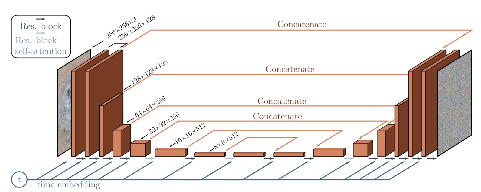
Score Architecture

• $\mathbf{s}_{\mathbf{\theta}}: \mathbb{R}^d\times [0,T] \rightarrow \mathbb{R}^d$ is a (complex) U-net (Ronneberger et al., 2015), eg in (Ho et al., 2020) "All models have two convolutional residual blocks per resolution level and self-attention blocks at the 16x16 resolution between the convolutional blocks".
• Diffusion time $t$ is specified by adding the Transformer sinusoidal position embedding into each residual block (Vaswani et al., 2017).

Exponential moving average

• Several choices for $t \mapsto \lambda_t$ (Kingma and Gao, 2023).
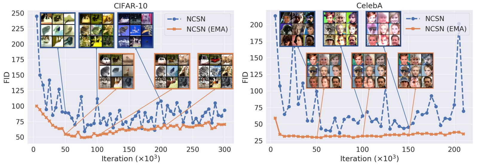
• Training using Adam algorithm (Kingma and Ba, 2015), but still unstable.
• To regularize: Exponential Moving Average (EMA) of weights. $$\bar{\theta}_{n+1} = (1-m)\bar{\theta}_{n} + m\theta_m$$
• Typically $m=10^{-4}$ (more than $10^4$ iterations are averaged).
• The final averaged parameters $\bar{\theta}_K$ are used at sampling.

Exponential moving average

Sampling Strategy

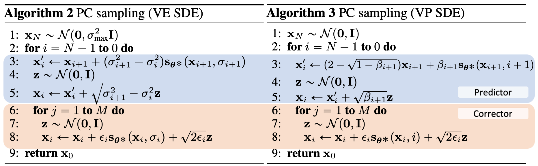
• The score function of a distribution is generally used for Langevin sampling. $$\mathbf{X}_{n+1} = \mathbf{X}_{n} + \gamma\nabla_{\mathbf{x}}\log p(\mathbf{X}_n) + \sqrt{2\gamma}\mathbf{Z}_n$$
• (Song et al., 2021b) propose to add one step of Langevin diffusion (same $t=t_n$) after each step Euler-Maruyama step ($t_n$ to $t_{n+1}$).
• This means that we jump from one trajectory to the other, but we correct some defaults from the Euler scheme.
• This is called a Predictor-Corrector sampler.

Sampling Strategy

Results

• (Song et al., 2021b) achieved SOTA in terms of FID for CIFAR-10 unconditional sampling.
• Very good results for 1024x1024 portrait images.
• See also "Diffusion Models Beat GANs on Image Synthesis"

Many approximations

• Many approximations in the full generative pipelines:
• The final distribution $p_T$ is not exactly a normal distribution.
• The learnt U-Net model $s_{\theta}$ is far from being the exact score function:
• Sample-based, limitations from the architecture...
• Discrete sampling scheme (Euler-Maruyama, Predictor-Corrector,...).
• Score function may behave badly near $t = 0$ (irregular density in case of manifold hypothesis).
• But we do have theoretical guarantees if all is well controlled.

Theorem (Convergence guarantees (De Bortoli, 2022)) Let $p_0$ be the data distribution having a compact manifold support and let $q_T$ be the generator distribution from the reversed diffusion. Under suitable hypotheses, the 1-Wasserstein distance $\mathcal{W}_1(p_0 , q_T)$ can be explicitly bounded and tends to zero when all the parameters are refined (more Euler steps, better score learning, etc.).

Sampling via an ODE

• We derived the Fokker-Plank equation for $q_t = p_{T-t}$ of reversed diffusion $y_t=x_{T-t}$.
$$ \begin{aligned} \partial_tq_t(\mathbf{x}) & = -\partial_t p_{T-t}(\mathbf{x}) \\ & = \nabla_{\mathbf{x}}(\mathbf{f}(\mathbf{x},T-t)p_{T-t}(\mathbf{x})) - \frac{1}{2}g(T-t)^2\nabla^2_{\mathbf{x}}p_{T-t}(\mathbf{x}) \\ & = \nabla_{\mathbf{x}}(\mathbf{f}(\mathbf{x},T-t)q_{t}(\mathbf{x})) - \frac{1}{2}g(T-t)^2\nabla^2_{\mathbf{x}}q_{t}(\mathbf{x}) \\ & = \nabla_{\mathbf{x}}(\mathbf{f}(\mathbf{x},T-t)p_{T-t}(\mathbf{x})) + \color{orange}{\left(-1 + \frac{1}{2}\right)} \frac{1}{2}g(T-t)^2\nabla^2_{\mathbf{x}}q_{t}(\mathbf{x}) \\ & = \nabla_{\mathbf{x}}\left([\mathbf{f}(\mathbf{x},T-t) + g(T-t)^2\nabla \log q_t(\mathbf{x})]q_{t}(\mathbf{x})\right) + \frac{1}{2}g(T-t)^2\nabla^2_{\mathbf{x}}q_{t}(\mathbf{x}) \end{aligned} $$
• This is the Fokker-Planck equation associated with the diffusion SDE: $$d\mathbf{y}_t = [-\mathbf{f}(\mathbf{y}_t,T-t)+g(T-t)^2\nabla_x\log p_{T-t}(\mathbf{y}_t)]dt + g(T-t)d\mathbf{w}_t$$

Sampling via an ODE

• We derived the Fokker-Plank equation for $q_t = p_{T-t}$ of reversed diffusion $y_t=x_{T-t}$.
$$ \begin{aligned} \partial_tq_t(\mathbf{x}) & = -\partial_t p_{T-t}(\mathbf{x}) \\ & = \nabla_{\mathbf{x}}(\mathbf{f}(\mathbf{x},T-t)p_{T-t}(\mathbf{x})) - \frac{1}{2}g(T-t)^2\nabla^2_{\mathbf{x}}p_{T-t}(\mathbf{x}) \\ & = \nabla_{\mathbf{x}}(\mathbf{f}(\mathbf{x},T-t)q_{t}(\mathbf{x})) - \frac{1}{2}g(T-t)^2\nabla^2_{\mathbf{x}}q_{t}(\mathbf{x}) \\ & = \nabla_{\mathbf{x}}(\mathbf{f}(\mathbf{x},T-t)p_{T-t}(\mathbf{x})) + \color{orange}{\left(-\frac{1}{2} + 0\right)} \frac{1}{2}g(T-t)^2\nabla^2_{\mathbf{x}}q_{t}(\mathbf{x}) \\ & = -\nabla_{\mathbf{x}}\left([-\mathbf{f}(\mathbf{x},T-t) + \frac{1}{2}g(T-t)^2\nabla \log q_t(\mathbf{x})]q_{t}(\mathbf{x})\right) \end{aligned} $$
• This is the Fokker-Planck equation associated with the diffusion SDE: $$d\mathbf{y}_t = [-\mathbf{f}(\mathbf{y}_t,T-t)+\frac{1}{2}g(T-t)^2\nabla_x\log p_{T-t}(\mathbf{y}_t)]dt$$ which is an Ordinary Differential Equation (ODE) (no stochastic term).

Reverse Diffusion via an ODE

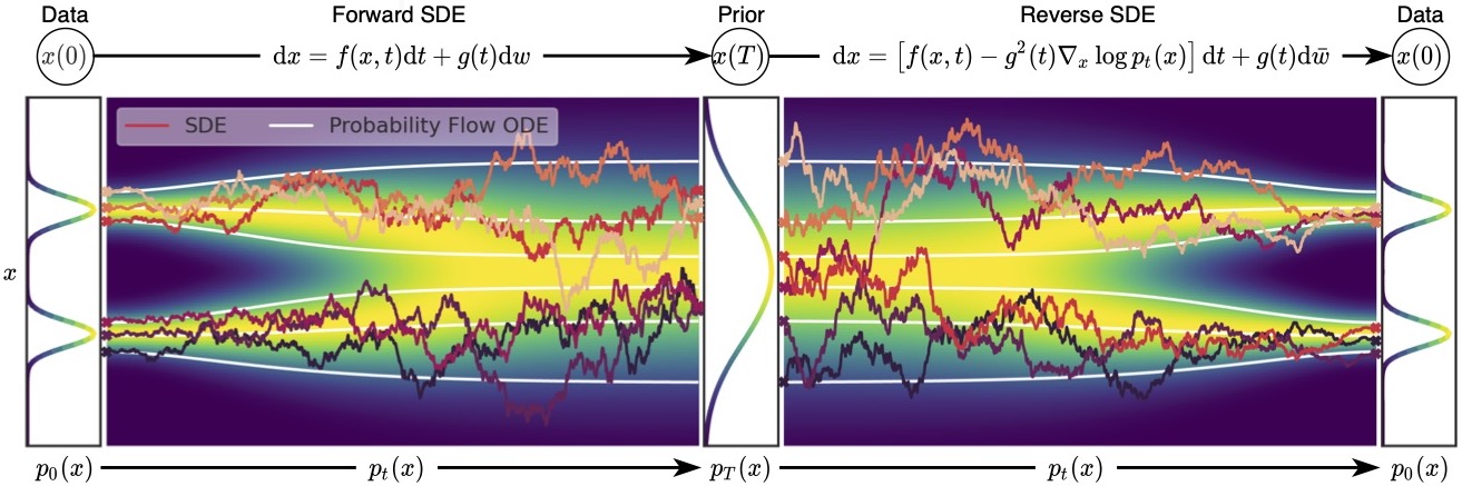
• We get a deterministic mapping between initial noise and generated images.
• We do not simulate the (chaotic) path of the stochastic diffusion but we still have the same marginal distribution $p_t$.
• We can use any ODE solver, with higher order than Euler scheme.

Reverse Diffusion via an ODE

• From (Karras et al., 2022) "Through extensive tests, we have found Heun's 2nd order method (a.k.a. improved Euler, trapezoidal rule) [...] to provide an excellent tradeoff between truncation error and NFE."
• Requires much less NFE than stochastic samplers (eg around 50 steps instead of 1000), see also Denoising Diffusion Implicit Models (DDIM) (Song et al., 2021a) for a deterministic approach.