Score Matching and Diffusion Models

Score Matching and Diffusion Models - III

CSE 849: Deep Learning

Vishnu Boddeti

Recap: Core Idea

Interpolating between two distributions:

The data distribution is denoted $p_{data} \in \mathcal{P}(\mathbb{R}_d)$.
The easy-to-sample distribution is denoted $p_{ref} \in \mathcal{P}(\mathbb{R}_d)$.
$p_{ref}$ is usually the standard multivariate Gaussian.

Going from the data to the easy-to-sample distribution: noising process.
Going from the easy-to-sample to the data distribution: generative process.
How to invert the forward noising process?

Denoising Diffusion Probabilistic Models

Denoising Diffusion Probabilistic Models (DDPM (Ho et al., 2020)) is a discrete model with a fixed number of $T=10^3$ steps that performs discrete diffusion.

Forward model: Discrete variance preserving diffusion (WARNING: Change of notation)

Distribution of samples: $q(\mathbf{x}_0)$.
Conditional Gaussian noise: $q(\mathbf{x}_t|\mathbf{x}_{t-1})=\mathcal{N}(\sqrt{1-\beta_t}\mathbf{x}_{t-1}, \beta_t\mathbf{I}_d)$ $$\mathbf{x}_t = \sqrt{1-\beta_t}\mathbf{x}_{t-1} + \beta_t\mathbf{z}_t$$ where the variance schedule $(\beta_t)_{1\leq t\leq T}$ is fixed.
One step noising $q(\mathbf{x}_t|\mathbf{x}_0)$: with $\alpha_t=1-\beta_t$ and $\bar{\alpha}=\text{cumulative product of } \alpha$ $$\mathbf{x}_t = \bar{\alpha}_t\mathbf{x}_0 + \sqrt{1-\bar{\alpha}_t}\mathbf{z}_t \text{ where } \mathbf{z} \text{ is standard.}$$

Diffusion Forward

Diffusion Backward

Diffusion parameters are designed such that $q(\mathbf{x}_T)\approx \mathcal{N}(\mathbf{0},\mathbf{I}_d)$

In general $q(\mathbf{x}_{t-1}|\mathbf{x}_t) \propto q(\mathbf{x}_{t-1})q(\mathbf{x}_t|\mathbf{x}_{t-1})$ is intractable.

Denoising Diffusion Probabilistic Models

We consider the diffusion as a fixed stochastic encoder.
We want to learn a stochastic decoder $p_{\theta}$: $$p_{\theta}(\mathbf{x}_{0:T}) = \underbrace{p(\mathbf{x}_T)}_{\text{fixed latent prior}}\prod_{t=1}^T\underbrace{p_{\theta}(\mathbf{x}_{t-1}|\mathbf{x}_t)}_{\text{learnable backward transitions}}$$ with $p_{\theta}(\mathbf{x}_{t-1}|\mathbf{x}_t) = \mathcal{N}(\mu_{\theta}(\mathbf{x}_t,t), \beta_t\mathbf{I}_d)$. $$\text{Compare with: } q(\mathbf{x}_t|\mathbf{x}_{t-1}) = \mathcal{N}(\sqrt{1-\beta_t}\mathbf{x}_{t-1}, \beta_t\mathbf{I}_d)$$
Recall same diffusion coefficient, new backward drift to be learnt.
Oversimplified version compared to (Ho et al., 2020), there are ways to also learn the variance for each pixel, see (Nichol and Dhariwal, 2021).
Then we look for training the decoder by maximizing an ELBO.

DDPM Training Loss

$$\mathbb{E}(-\log p_{\theta}(\mathbf{x}_0)) \leq \mathbb{E}_q\left[-\log\left[\frac{p_{\theta}(\mathbf{x}_{0:T})}{q(\mathbf{x}_{1:T}|\mathbf{x}_0)}\right]\right] := L$$

We have

$$ \begin{aligned} L &= \mathbb{E}_q\left[-\log p(\mathbf{x}_T) - \sum_{t=1}^T \log \frac{p_{\theta}(\mathbf{x}_{t-1}|\mathbf{x}_t)}{q(\mathbf{x}_t|\mathbf{x}_{t-1})}\right]\\ &= \mathbb{E}_q\left[D_{KL}(q(\mathbf{x}_t|\mathbf{x}_0)\|p(\mathbf{x}_T)) + \sum_{t=2}^T D_{KL}(q(\mathbf{x}_{t-1}|\mathbf{x}_t,\mathbf{x}_0)\|p_{\theta}(\mathbf{x}_{t-1}|\mathbf{x}_t)) - \log p_{\theta}(\mathbf{x}_0|\mathbf{x}_1)\right] \end{aligned} $$

DDPM: Training Loss continued...

Computation of $D_{KL}(q(\mathbf{x}_{t-1}|\mathbf{x}_t,\mathbf{x}_0)\|p_{\theta}(\mathbf{x}_{t-1}|\mathbf{x}_t))$
By Bayes rule, $$q(\mathbf{x}_{t-1}|\mathbf{x}_t,\mathbf{x}_0)=q(\mathbf{x}_t|\mathbf{x}_{t-1},\mathbf{x}_0)\frac{q(\mathbf{x}_{t-1}|\mathbf{x}_0)}{q(\mathbf{x}_t|\mathbf{x}_0)} = q(\mathbf{x}_t|\mathbf{x}_{t-1})\frac{q(\mathbf{x}_{t-1}|\mathbf{x}_0)}{q(\mathbf{x}_t|\mathbf{x}_0)}$$
Computation shows that this is a normal distribution $\mathcal{N}(\tilde{\mu}(\mathbf{x}_t,\mathbf{x}_0),\tilde{\beta}\mathbf{I}_d)$ with $$\tilde{\mu}(\mathbf{x}_t,\mathbf{x}_0)=\frac{\sqrt{\bar{\alpha}_{t-1}}\beta_t}{1-\bar{\alpha}_t}\mathbf{x}_0 + \frac{\sqrt{\alpha_t}(1-\bar{\alpha}_{t-1})}{1-\bar{\alpha}_t}\mathbf{x}_t \text{ and } \tilde{\beta}_t=\frac{1-\bar{\alpha}_{t-1}}{1-\bar{\alpha}}\beta_t$$
Using the expression of the KL-divergence between Gaussian distributions, $$D_{KL}(q(\mathbf{x}_{t-1}|\mathbf{x}_t,\mathbf{x}_0)\|p_{\theta}(\mathbf{x}_{t-1}|\mathbf{x}_t)) = \frac{1}{\beta_t}\|\mu_{\theta}(\mathbf{x}_t,t) - \tilde{\mu}(\mathbf{x}_t,\mathbf{x}_0)\|^2 + C$$

$$L_t = \mathbb{E}_q[D_{KL}(q(\mathbf{x}_{t-1}|\mathbf{x}_t,\mathbf{x}_0)\|p_{\theta}(\mathbf{x}_{t-1}|\mathbf{x}_t))] = \frac{1}{\beta_t}\mathbb{E}_q\left[\|\mu_{\theta}(\mathbf{x}_t,t) - \tilde{\mu}(\mathbf{x}_t,\mathbf{x}_0)\|^2\right] + C$$

DDPM: Noise reparameterization

Rewrite everything as a function of the added noise $\epsilon$ $$\mathbf{x}_t(\mathbf{x}_0,\epsilon) = \sqrt{\bar{\alpha}_t}\mathbf{x}_0 + \sqrt{1-\bar{\alpha}_t}\epsilon$$
Then $\mu_{\theta}(\mathbf{x}_t,t)$ must predict $$\tilde{\mu}(\mathbf{x}_t,\mathbf{x}_0)=\frac{1}{\sqrt{\alpha_t}}\left(\mathbf{x}_t - \frac{\beta_t}{\sqrt{1-\bar{\alpha}_t}}\mathbf{\epsilon}\right)$$
If we parameterize $$\mu_{\theta}(\mathbf{x}_t,t) = \frac{1}{\sqrt{\alpha_t}}\left(\mathbf{x}_t - \frac{\beta_t}{\sqrt{1-\bar{\alpha}_t}}\mathbf{\epsilon_{\theta}(\mathbf{x}_t,t)}\right)$$
Then the loss is simply $$ \begin{aligned} L_t &= \frac{\beta_t}{1-\bar{\alpha}_t}\mathbb{E}_q\left[\|\epsilon_{\theta}(\mathbf{x}_t,t) - \epsilon\|^2\right] + C \\ & = \frac{\beta_t}{1-\bar{\alpha}_t}\mathbb{E}_q\left[\|\epsilon_{\theta}(\sqrt{\bar{\alpha}_t}\mathbf{x}_0 + \sqrt{1-\bar{\alpha}_t}\epsilon,t) - \epsilon\|^2\right] + C \end{aligned} $$
We must predict the noise $\epsilon$ added to $\mathbf{x}_0$ (without knowing $\mathbf{x}_0$).

DDPM: Training and sampling

$$ \begin{aligned} L &= \mathbb{E}_q\left[D_{KL}(q(\mathbf{x}_T|\mathbf{x}_0)\|p(\mathbf{x}_T)) + \sum_{t=2}^TD_{KL}(q(\mathbf{x}_{t-1}|\mathbf{x}_t,\mathbf{x}_0)\|p(\mathbf{x}_{t-1}|\mathbf{x}_t)) - \log p_{\theta}(\mathbf{x}_0|\mathbf{x}_1)\right] \\ &= \sum_{t=2}^T L_t + L_1 + C \end{aligned} $$

The $L_1$ term is dealt differently (to account for discretization of $\mathbf{x}_0$).
(Ho et al., 2020) proposes to simplify the loss (no constants): $$L_{simple} = \mathbb{E}_{t,\mathbf{x}_0,\mathbf{\epsilon}}\left[\|\mathbf{\epsilon}_{\theta}(\sqrt{\bar{\alpha}}\mathbf{x}_0 + \sqrt{1-\bar{\alpha}_t}\mathbf{\epsilon}, t) - \mathbf{\epsilon}\|\right]$$

DDPM: Training and sampling

$\sigma_t = \sqrt{\beta_t}$ here.

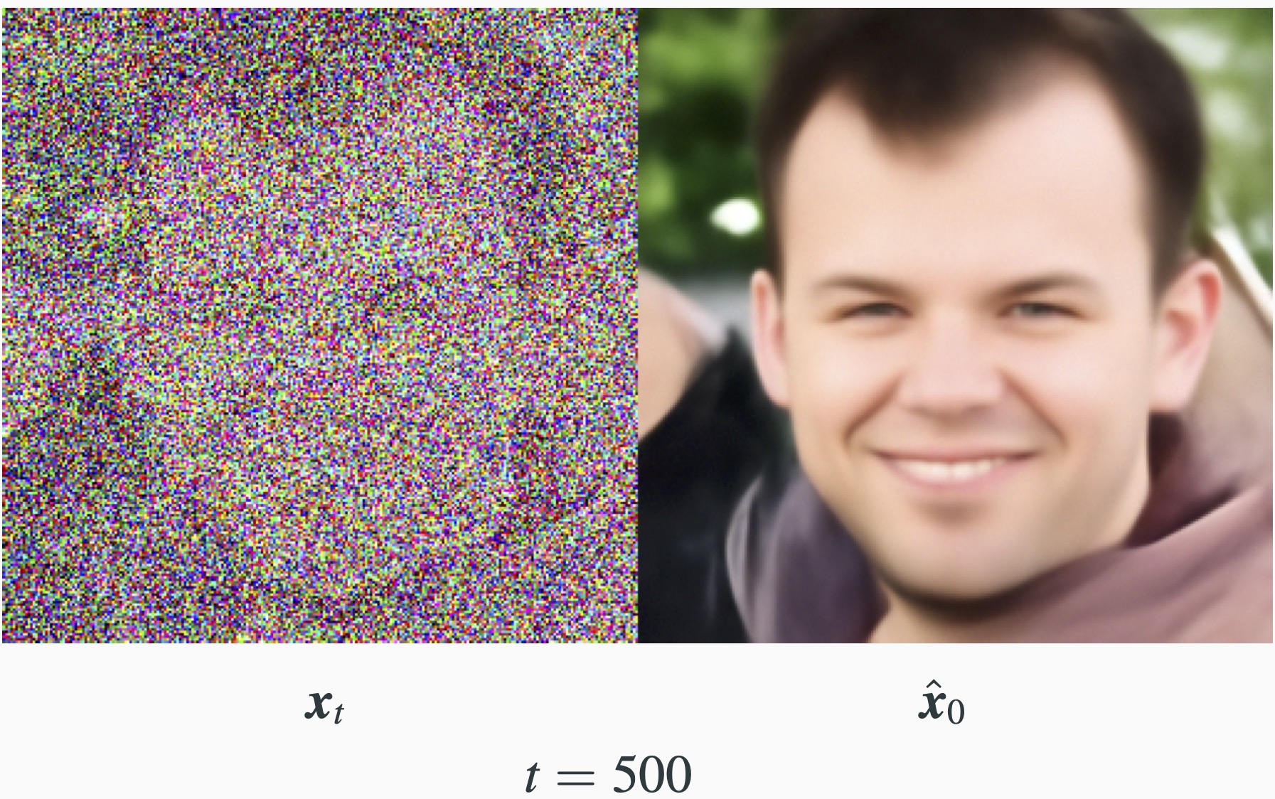
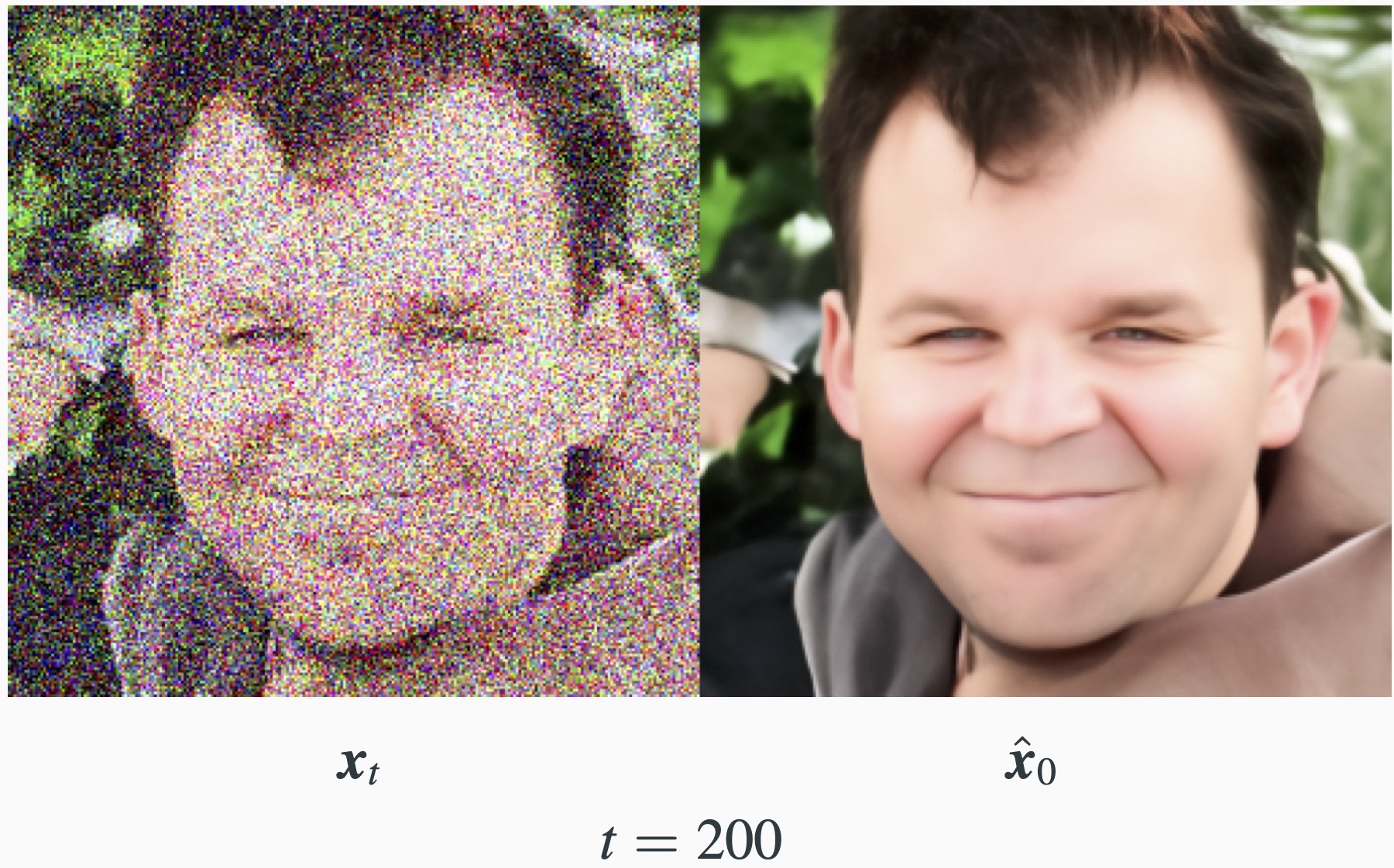
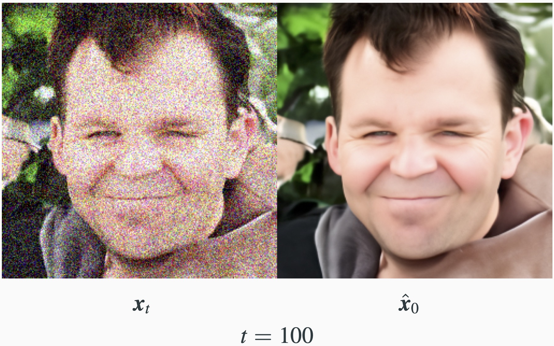
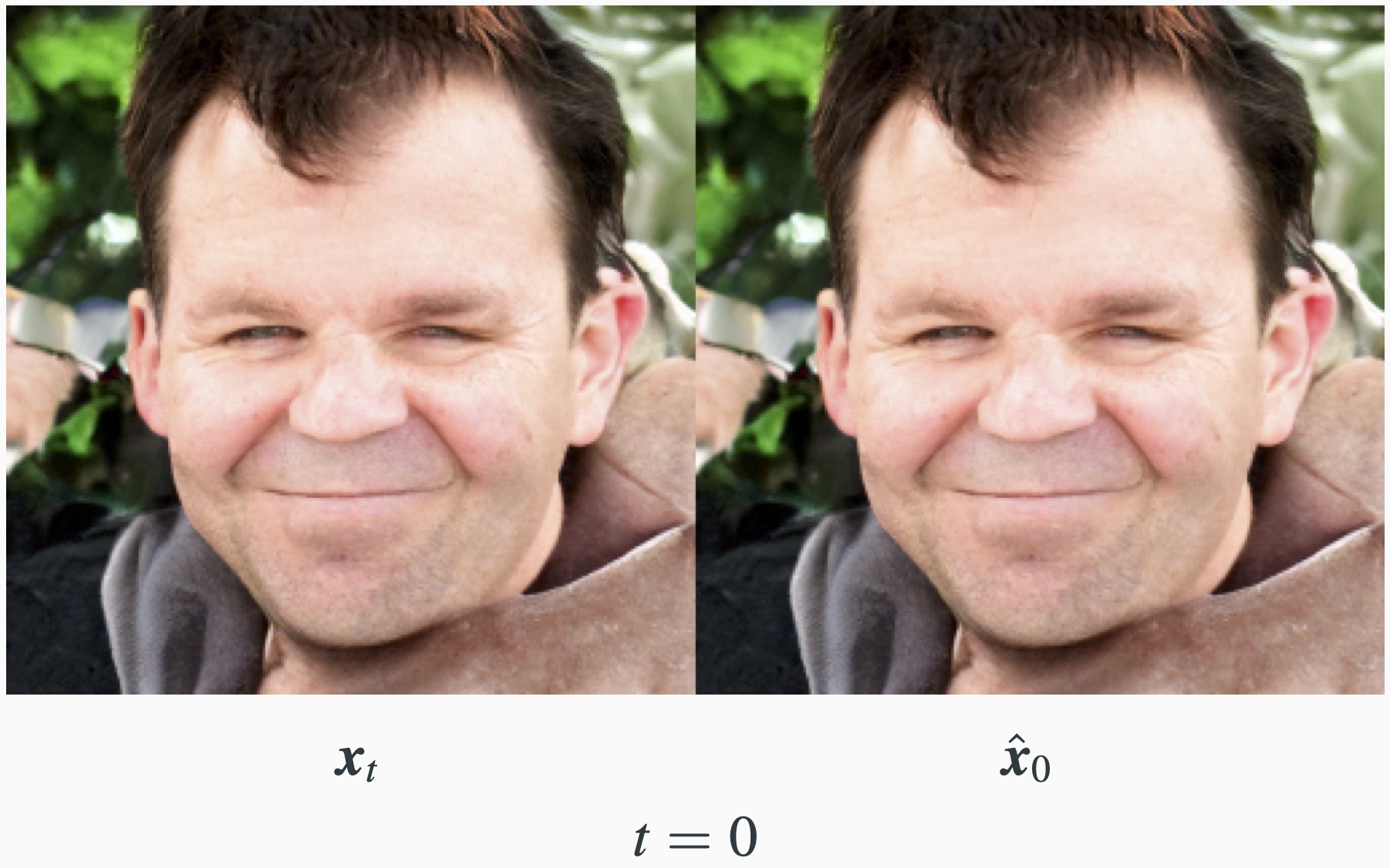
DDPM: Denoiser

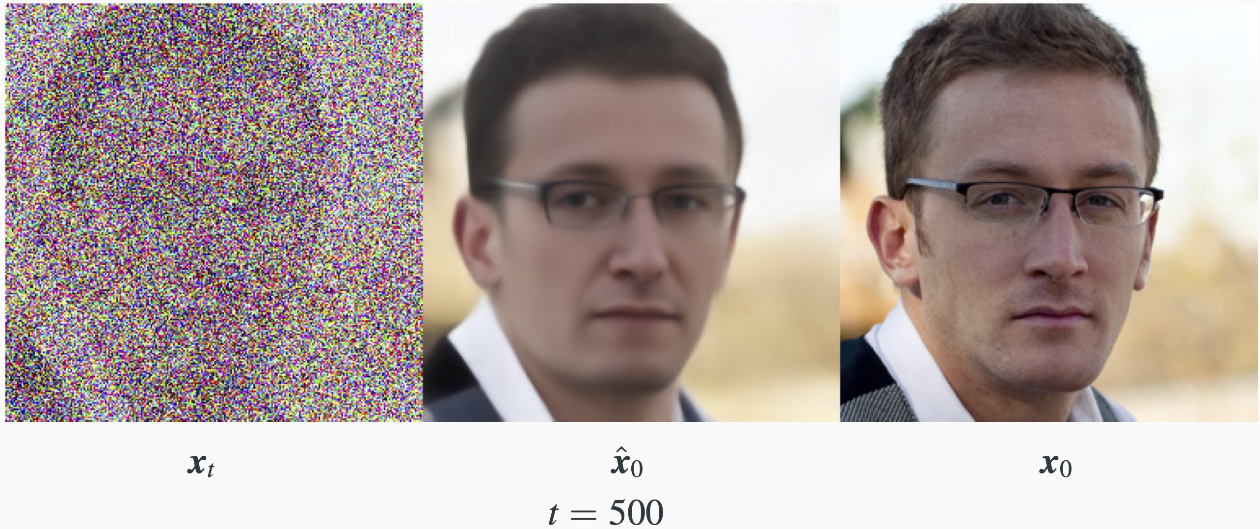
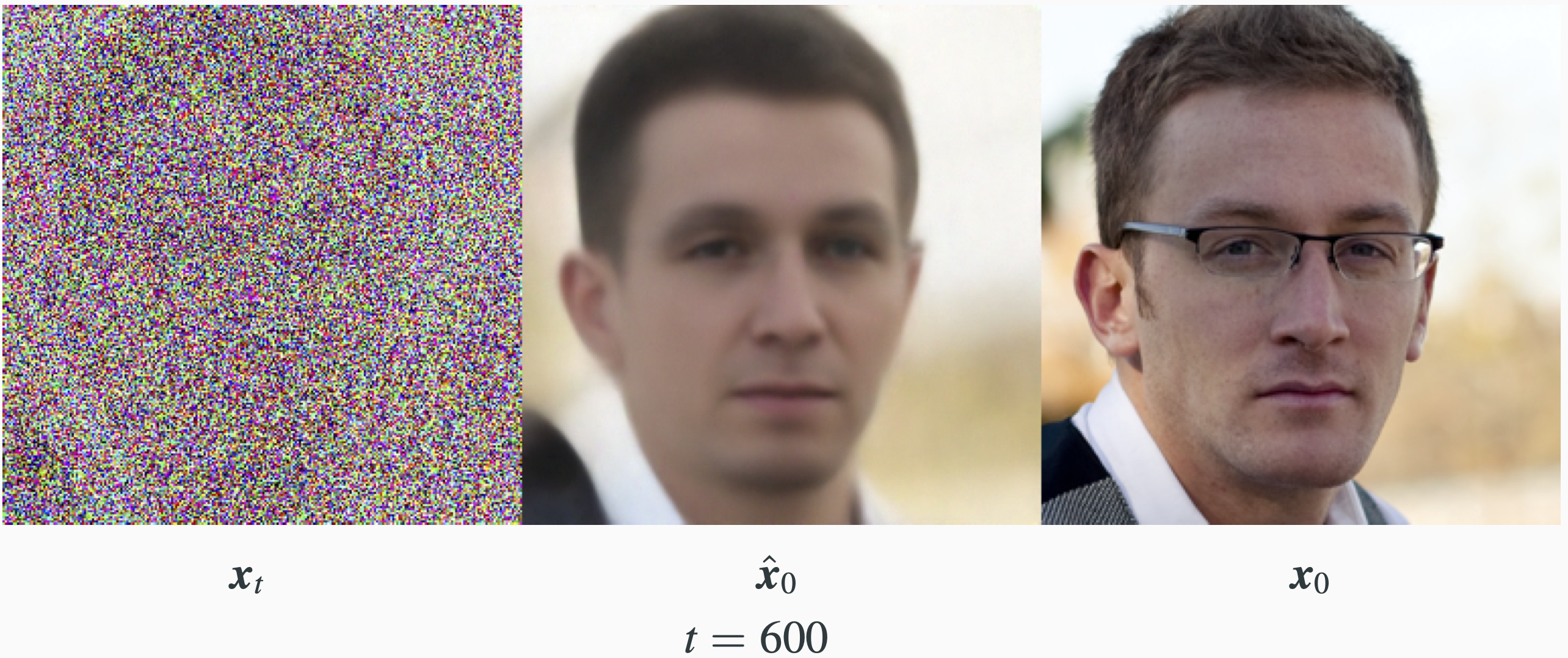
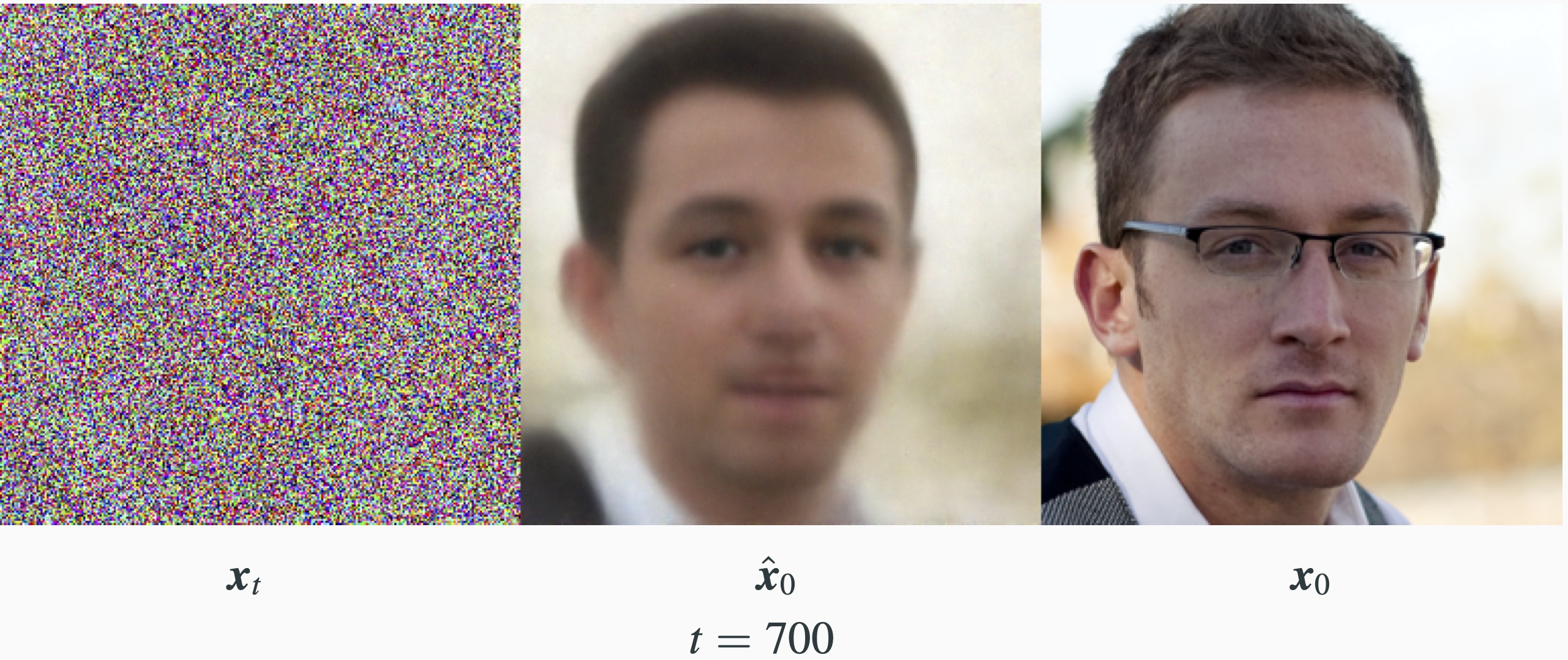
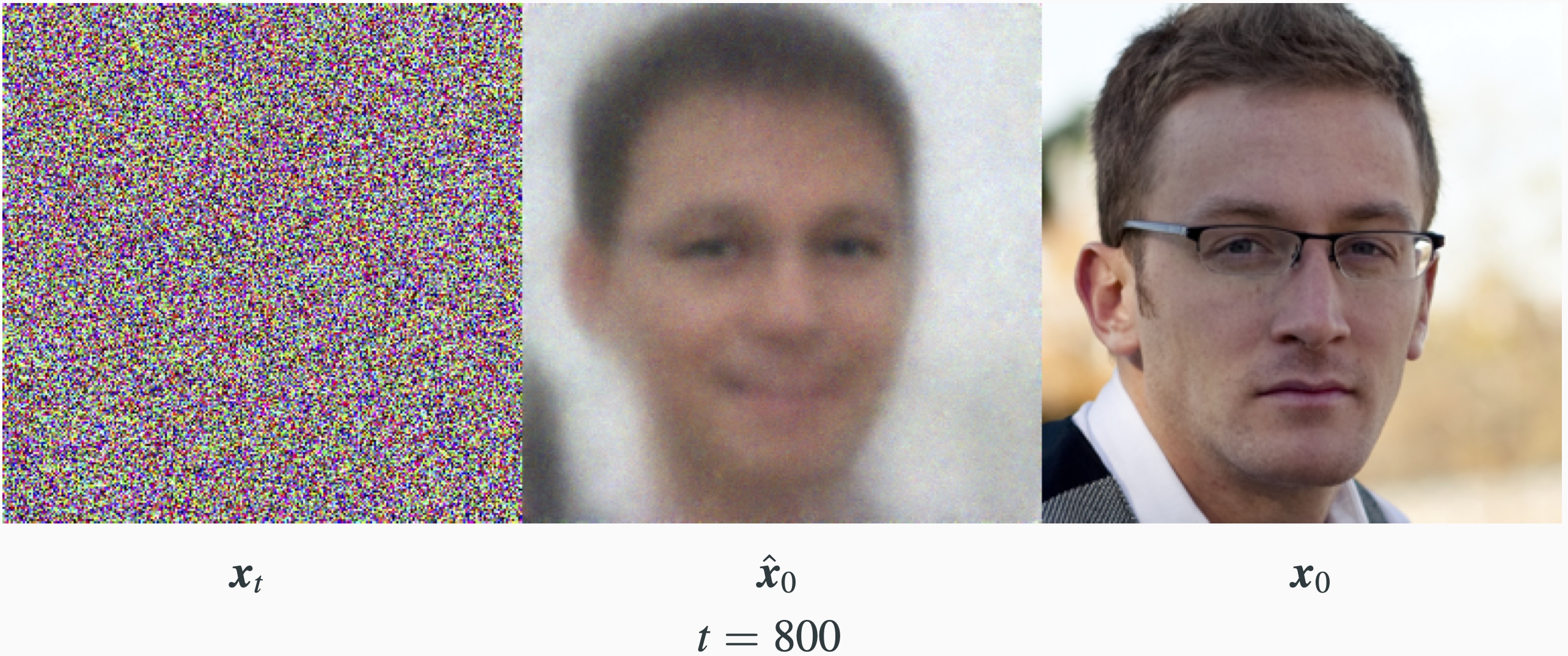
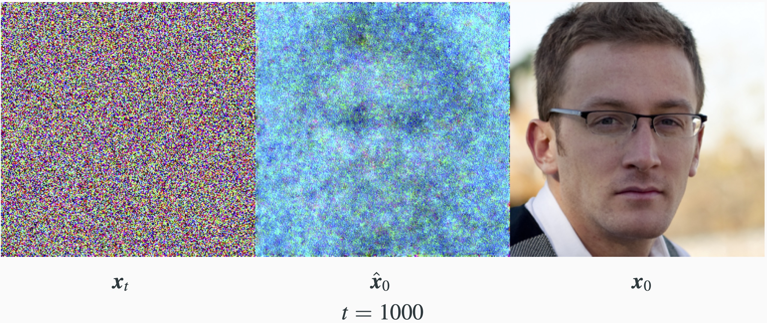
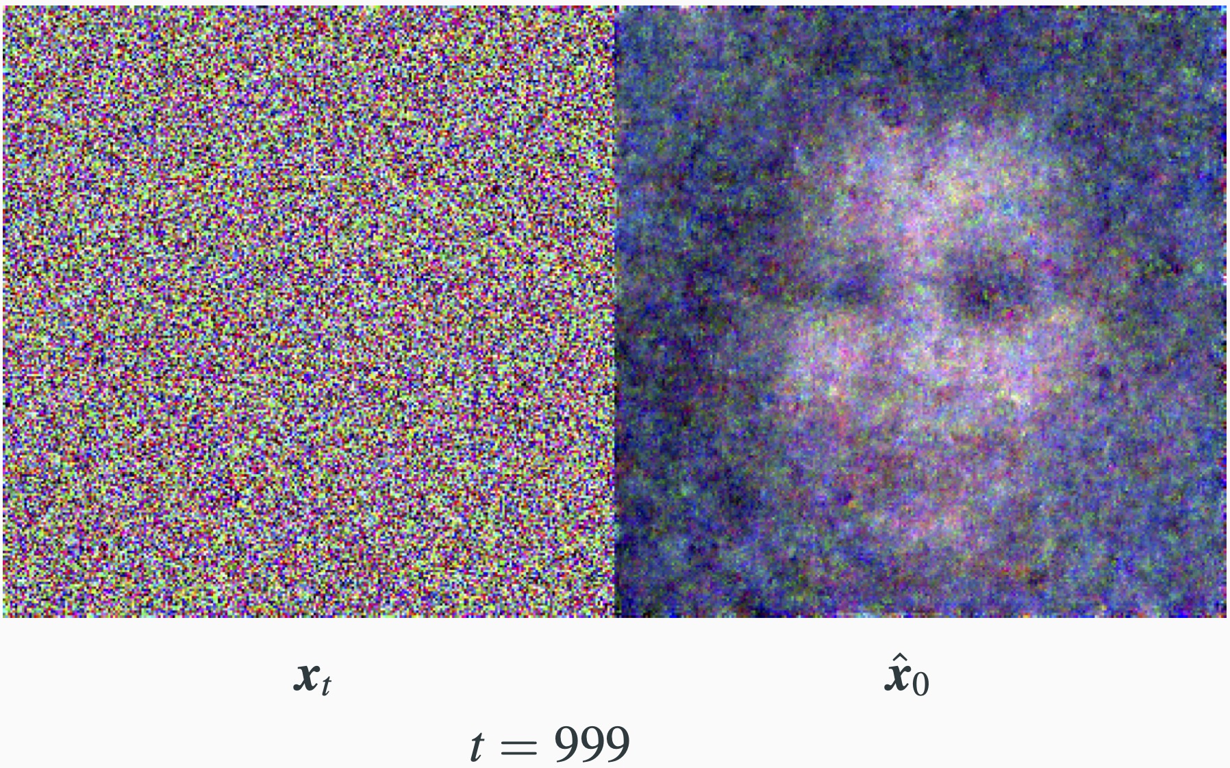
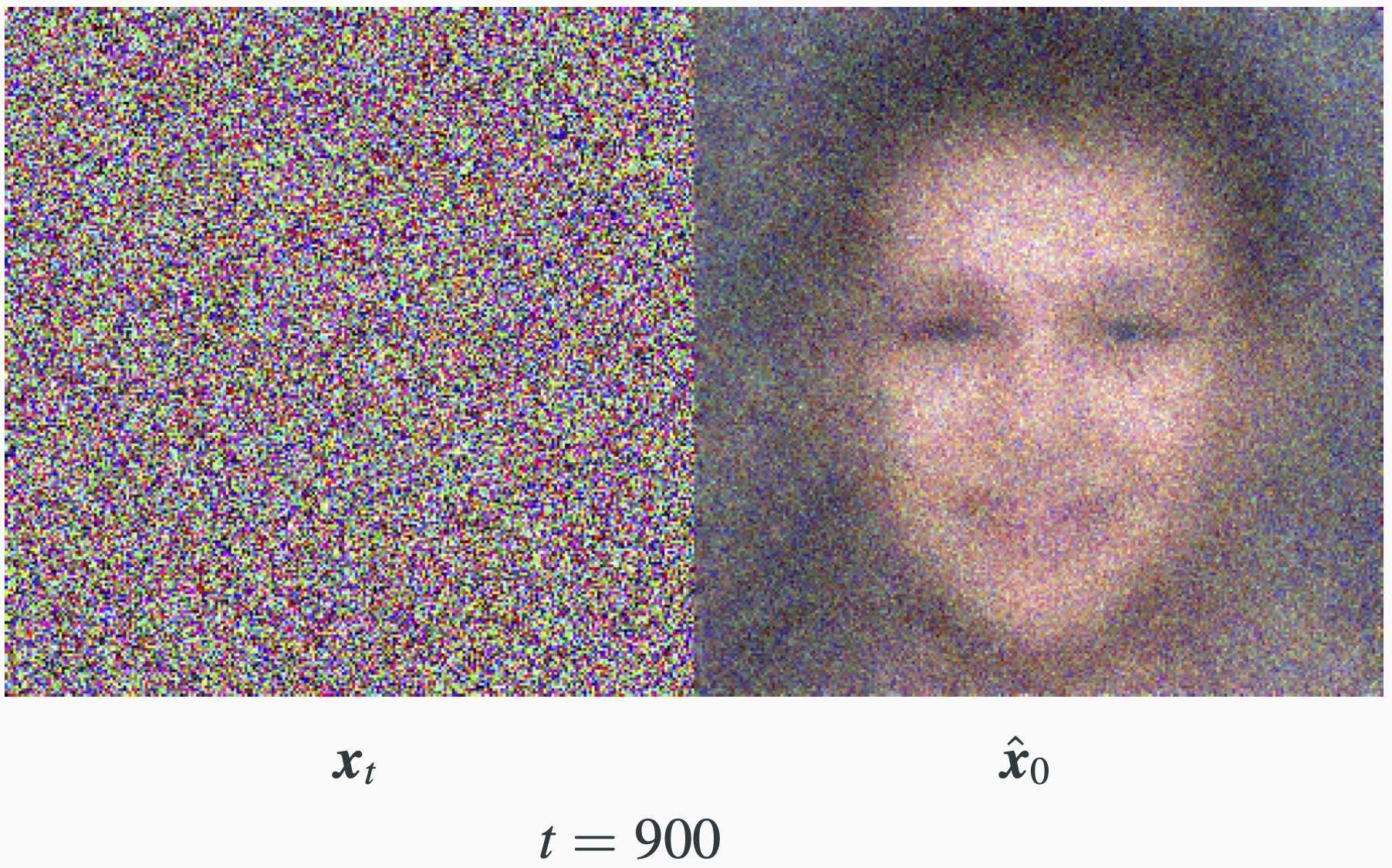
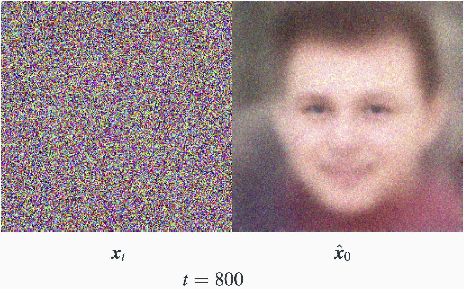
The U-Net $\epsilon_{\theta}(\mathbf{x}_t,t)$ is a (residual) denoiser that gives an estimation of the noise $\epsilon$ from $$\mathbf{x}_t(\mathbf{x}_0,\epsilon)=\sqrt{\bar{\alpha}_t}\mathbf{x}_0 + \sqrt{1-\bar{\alpha}_t}\epsilon.$$
We get the associated estimation of $\mathbf{x}_0$: $$\hat{\mathbf{x}}_0 = \frac{1}{\sqrt{\bar{\alpha}}_t}\mathbf{x}_t - \sqrt{\frac{1}{\bar{\alpha}_t}-1}\epsilon_{\theta}(\mathbf{x}_t,t).$$

DDPM: Sampling

$\sigma_t = \sqrt{\beta_t}$ here.

Score Matching vs DDPM

Score Matching and DDPM

Diffusion model via SDE: (Song et al., 2021)

Diffusion model via Denoising Diffusion Probabilistic Models (DDPM): (Ho et al., 2020) Discrete model with a fixed number of $T=10^3$.

Score Matching vs DDPM

$$ d\mathbf{x}_t = \mathbf{f}(\mathbf{x}_t, t)dt + g(t)d\mathbf{w}_t$$

Example 1: Variance exploding diffusion (VE-SDE) $$ \begin{aligned} \text{SDE:} & \quad d\mathbf{x}_t = d\mathbf{w}_t \\ \text{Solution:} & \quad \mathbf{x}_t = \mathbf{x}_0 + \mathbf{w}_t \\ \text{Variance:} & \quad Var(\mathbf{x}_t) = Var(\mathbf{x}_0) + t \end{aligned} $$
Example 2: Variance preserving diffusion (VP-SDE) $$ \begin{aligned} \text{SDE:} & \quad \mathbf{x}_t = -\beta_t\mathbf{x}_tdt + \sqrt{2\beta_t}d\mathbf{w}_t \\ \text{Solution:} & \quad \mathbf{x}_t = e^{-B_t}\mathbf{x}_0 + \int_{0}^te^{B_2-B_t}\sqrt{2\beta_s}d\mathbf{w}_s \text{ with } B_t=\int_{0}^t\beta_tdt \\ \text{Variance:} & \quad Var(\mathbf{x}_t) = e^{-2B_t}Var(\mathbf{x}_0) + 1 - e^{-2B_t} \end{aligned} $$
Both variants have the form $\mathbf{x}_t = \alpha_t \mathbf{x}_0 + \beta_t \mathbf{Z}_t: \mathbf{x}_t$ is a rescaled noisy version of $\mathbf{x}_0$ and the noise is more and more predominant as time grows.

Continuous Diffusion Models

Forward diffusion: $$d\mathbf{x}_t = \mathbf{f}(\mathbf{x}_t, t)dt + g(t)d\mathbf{w}_t$$
Backward diffusion: $\mathbf{y}_t = \mathbf{x}_{T-t}$ $$d\mathbf{y}_t = -\mathbf{f}(\mathbf{y}_t, T-t)dt + g(T-t)d\mathbf{w}_t$$

Learn score by denoising score matching: $$\theta^{*} = arg\min \mathbb{E}_t\left(\lambda_t\mathbb{E}_{(\mathbf{x}_0, \mathbf{x}_t)}\|s_{\theta}(\mathbf{x}_t,t) - \nabla_{\mathbf{x}_t}\log p_{t|0}(\mathbf{x}_t|\mathbf{x}_0)\|^2\right) \text{ with } t \sim U([0,T])$$
Generate samples by SDE discrete scheme (e.g. Euler-Maruyama): $$\mathbf{Y}_{n-1} = \mathbf{Y}_n - hf(\mathbf{Y}_n, t_n) +hg(t_n)^2\mathbf{s}_{\theta}(\mathbf{Y}_n, t_n) + g(t_n)\sqrt{h}\mathbf{Z}_n \text{ with } \mathbf{Z}_n \sim \mathcal{N}(\mathbf{0}, \mathbf{I}_d)$$
Associated deterministic probability flow: $$d\mathbf{y}_t = \left[-\mathbf{f}(\mathbf{y}_t, T-t) + \frac{1}{2}g(T-t)^2\nabla_{\mathbf{x}}\log p_{T-t}(\mathbf{y}_t)\right]dt$$

Denoising Diffusion Probabilistic Models (DDPM)

Forward Diffusion:
Backward diffusion: stochastic decoder $p_{\theta}$: $$p_{\theta}(\mathbf{x}_{0:T}) = \underbrace{p(\mathbf{x}_T)}_{\text{fixed latent prior}}\prod_{t=1}^T\underbrace{p_{\theta}(\mathbf{x}_{t-1}|\mathbf{x}_t)}_{\text{learnable backward transitions}} \text{ with } \underbrace{p_{\theta}(\mathbf{x}_{t-1}|\mathbf{x}_t) = \mathcal{N}(\mu_{\theta}(\mathbf{x}_t,t), \beta_t\mathbf{I}_d)}_{\text{Gaussian approximation of } q(\mathbf{x}_{t-1}|\mathbf{x}_t)}$$

Denoising Diffusion Probabilistic Models (DDPM)

Learn the score by minimizing the ELBO (like for VAE): This boils down to denoising the diffusion iterations $\mathbf{x}_t = \sqrt{\bar{\alpha}}\mathbf{x}_0 + \sqrt{1-\bar{\alpha}}\epsilon$ $$\theta^{*} = arg\min\sum_{t=1}^T \frac{\beta_t}{1-\bar{\alpha}_t}\mathbb{E}_q\left[\|\mathbf{\epsilon}_{\theta}(\mathbf{x}_t, t)-\mathbf{\epsilon}\|^2\right] + C$$
Sampling through the stochastic decoder with $$ \mu_{\theta}(\mathbf{x}_t, t) = \frac{1}{\sqrt{\alpha_t}}\left(\mathbf{x}_t - \frac{\beta_t}{\sqrt{1-\bar{\alpha}_t}}\epsilon_{\theta}(\mathbf{x}_t, t)\right)$$

DDPM Training and Score Matching

Posterior mean training: Recall that $\mu_{\theta}(\mathbf{x}_t,t)$ minimizes $$ \mathbb{E}_q[D_{KL}(q(\mathbf{x}_{t-1}|\mathbf{x}_t)\|p_{\theta}(\mathbf{x}_{t-1}|\mathbf{x}_t))] = \frac{1}{\beta_t}\mathbb{E}_{q}\left[\|\mu_{\theta}(\mathbf{x}_t,t)-\tilde{\mu}(\mathbf{x}_t,\mathbf{x}_0)\|^2\right] + C$$ where $\tilde{\mu}(\mathbf{x}_t,\mathbf{x}_0)$ is the mean of $q(\mathbf{x}_{t-1}|\mathbf{x}_t,\mathbf{x}_0)$. Hence ideally, $$\mu_{\theta}(\mathbf{x}_t,t) = \mathbb{E}[\tilde{\mu}(\mathbf{x}_t,\mathbf{x}_0|\mathbf{x}_t)] = \mathbb{E}[\mathbb{E}[\mathbf{x}_{t-1}|\mathbf{x}_t,\mathbf{x}_0]|\mathbf{x}_t] = \mathbb{E}[\mathbf{x}_{t-1}|\mathbf{x}_t]$$
Noise prediction training: $\epsilon_{\theta}(\mathbf{x}_t,t)$ minimizes $$\mathbb{E}\left[\|\epsilon_{\theta}(\mathbf{x}_t,t)-\epsilon\|^2\right]$$ where $\epsilon$ is a function of $(\mathbf{x}_t,\mathbf{x}_0)$ since $\mathbf{x}_t=\sqrt{\bar{\alpha}}\mathbf{x}_0+\sqrt{1-\bar{\alpha}}\epsilon$. Hence ideally, $$\epsilon_{\theta}(\mathbf{x}_t,t) = \mathbb{E}[\epsilon|\mathbf{x}_t]$$
Score matching training: Ideally, $$s_{\theta}(\mathbf{x}_t,t) = \nabla_{\mathbf{x}_t}\log p_t(\mathbf{x}_t) = \mathbb{E}[\nabla_{\mathbf{x}_t}\log p_t(\mathbf{x}_t|\mathbf{x}_0)|\mathbf{x}_t]$$

Tweedie Formulae

We derived the formulae for DDPM training without considering the score function.
But denoising and score functions are linked by Tweedie formulae:

Tweedie Formulae

Theorem (Tweedie Formulae)

If $Y=aX + \sigma Z$ with $Z\sim\mathcal{N}(0, I_d)$ independent of $X$, $a > 0, \sigma > 0$, then
$$ \begin{aligned} \text{Tweedie denoiser:} & \quad \mathbb{E}[X|Y] = \frac{1}{a}\left(Y + \sigma^2\nabla_Y\log p_Y(Y)\right) \\ \text{Tweedie noise predictor:} & \quad \mathbb{E}[Z|Y] = -\sigma\nabla_{\mathbf{y}}\log p_Y(Y) \end{aligned} $$

DDPM and Tweedie

If $Y=aX + \sigma Z$ with $Z\sim\mathcal{N}(0, I_d)$ independent of $X$, $a > 0, \sigma > 0$, then $$ \begin{aligned} \text{Tweedie denoiser:} & \quad \mathbb{E}[X|Y] = \frac{1}{a}\left(Y + \sigma^2\nabla_Y\log p_Y(Y)\right) \\ \text{Tweedie noise predictor:} & \quad \mathbb{E}[Z|Y] = -\sigma\nabla_{\mathbf{y}}\log p_Y(Y) \end{aligned} $$

Tweedie for noise prediction: Predict the noise $\epsilon$ from $\mathbf{x}_t$: $$\mathbf{x}_t = \sqrt{\bar{\alpha}_t}\mathbf{x}_0 + \sqrt{1-\bar{\alpha}_t}\epsilon \Rightarrow \color{orange}{\mathbb{E}[\mathbf{\epsilon}|\mathbf{x}_t] = -\sqrt{1-\bar{\alpha}}\nabla_{\mathbf{x}_t}\log p_t(\mathbf{x}_t)}$$
Tweedie for one-step denoising: Predict $\mathbf{x}_{t-1}$ from $\mathbf{x}_t$: $$\mathbf{x}_t = \sqrt{\alpha_t}\mathbf{x}_{t-1} + \sqrt{\beta_t}\mathbf{z}_t \Rightarrow \mathbb{E}[\mathbf{x}_{t-1}|\mathbf{x}_t] = \frac{1}{\sqrt{\alpha}_t}\left(\mathbf{x}_t + \beta_t \nabla_{\mathbf{x}_t}\log p_t(\mathbf{x}_t)\right)$$ $$\color{orange}{\mathbb{E}[\mathbf{x}_{t-1}|\mathbf{x}_t] = \frac{1}{\sqrt{\alpha}_t}\left(\mathbf{x}_t - \frac{\beta_t}{\sqrt{1-\bar{\alpha}_t}}\mathbb{E}[\mathbf{\epsilon}|\mathbf{x}_t]\right)}$$ $$\mu_{\theta}(\mathbf{x}_t,t)=\frac{1}{\sqrt{\alpha_t}}\left(\mathbf{x}_t - \frac{\beta_t}{\sqrt{1-\bar{\alpha}_t}}\epsilon_{\theta}(\mathbf{x}_t,t)\right)$$

Summary of Diffusion Models

The two training strategies are the same (up to weighting constants)
The only difference between the continuous SDE model and the discrete DDPM model are the time values: $t \in [0, T]$ vs. $t = 1, \dots, T=10^3$.
Good news: We can train a DDPM and use it for a deterministic probability flow ODE (this is what is done by the DDIM model (Song et al., 2021)).