Higher-Order Derivatives in Modern AI

Training faster, opening the model, and tracing its data

Vishnu Boddeti

Jacobian or Hessian?

Jacobian: input–output sensitivity

$J_f(x)=[\partial f_i/\partial x_j]$

One row per output; one column per input.

Which input directions move the representation?

Hessian: local curvature

$H_f(\theta)=\nabla_\theta^2 f(\theta)$

It measures how the gradient changes as parameters move.

Which parameter directions are sharp or flat?

At model scale: use operators

$Jv,\quad u^\top J,\quad Hv$

Automatic differentiation applies these maps without storing the full matrix.

Ask for the product you need.

Pearlmutter, “Fast Exact Multiplication by the Hessian,” Neural Computation, 1994.

Example 1

Sophia uses curvature to pretrain language models faster

Estimate diagonal curvature

Scale each coordinate

Clip unsafe updates

Concrete exampleA GPT parameter in a sharp direction should move less than one in a flat direction, even when their gradients have similar magnitudes.

A single learning rate cannot adapt to strongly different curvatures across billions of parameters.

Sophia: A Scalable Stochastic Second-order Optimizer for Language Model Pre-training (Liu et al., 2023)

What problem does Sophia solve?

Sophia and AdamW validation loss curves for GPT-2 and GPT-NeoX pretraining, plus scaling with model size

Across the reported GPT-2 and GPT-NeoX runs, Sophia reaches the same validation loss in about half as many steps as AdamW.

Liu et al., “Sophia,” 2023, Figure 1. Figure reproduced from the paper.

Sophia keeps a cheap diagonal view of the Hessian

1. GradientAverage the noisy minibatch gradients.$m_t\approx\mathbb E[g_t]$

2. CurvatureOccasionally estimate the positive diagonal Hessian.$h_t\approx\operatorname{diag}(H_t)$

3. PreconditionDivide each coordinate by its own curvature scale.$m_t/(\gamma h_t+\varepsilon)$

4. ClipCap coordinates when curvature is noisy or negative.$\operatorname{clip}(\cdot,\rho)$

The second-order information is deliberately incomplete: Sophia trades a full Hessian for an inexpensive diagonal estimate refreshed only every few steps.

Increase curvature contrast and compare one learning rate with Hessian scaling

Move the control: one global step size becomes harder to tune as curvature becomes less uniform.

Sharp-to-flat curvature contrast

Second-order scaling lets sharp and flat coordinates make useful progress together.

Example 2

Neural-VSI recovers hidden fields in high-order PDEs

Measure a vibrating beam

Build local weak equations

Recover stiffness and damping

Concrete exampleFrom noisy displacement measurements, infer spatially varying stiffness P(x) and damping C(x) without knowing the boundary conditions.

The weak form moves high-order derivatives away from the learned field and turns repeated automatic differentiation into reusable matrix operations.

Neural-VSI: Variational System Identification of Structural Parameter Fields in High-Order PDEs (Li et al., 2026)

What problem does Neural-VSI solve?

Neural-VSI runtime and recovered stiffness and damping fields compared with a strong-form baseline

The task is system identification: recover the beam's hidden parameter fields from observed motion. The figure shows runtime, stiffness recovery, and damping recovery.

Li et al., “Neural-VSI,” ICLR AI&PDE Workshop, 2026, Figure 1.

The weak form changes what must be differentiated

Measured fieldSensors provide noisy displacement values.$u(x,t)$

Strong PDEThe beam equation contains fourth-order spatial derivatives.$\partial_x^2(Pu_{xx})$

Local weak formIntegration by parts transfers derivatives to known test functions.$\int_{\Omega_i}w\,\mathcal L[u]\,dx$

Parameter fieldsReusable matrices constrain neural fields for stiffness and damping.$P_\phi(x),\ C_\psi(x)$

The model still learns unknown functions, but it no longer asks automatic differentiation to repeatedly construct the highest-order spatial derivatives of the measured field.

Widen the weak-form window and trade spatial detail for noise averaging

A larger local window pools more measurements but blurs rapid spatial changes.

Local weak-form window size

The weak form is not merely faster: it changes the statistical and numerical problem the learner sees.

Example 3

A Jacobian turns one LLM prediction into a local linear map

Fix one prompt

Differentiate output embeddings

Inspect singular directions

Concrete exampleFor the prompt ‘The bridge out of Marin is the ...’, a Jacobian maps token-embedding perturbations to the next-token output embedding.

The full model is nonlinear, but its input-specific linear map exposes rank, sensitive directions, and semantic features for that prediction.

Equivalent Linear Mappings of Large Language Models (Golden, 2025)

What does an input-specific LLM Jacobian reveal?

Transformer diagram showing detached nonlinear gates and a Jacobian reconstruction of the predicted output embedding

Freeze the prompt-dependent gates during differentiation: the resulting Jacobian reconstructs the output embedding and can be decomposed with SVD.

Golden, “Equivalent Linear Mappings of Large Language Models,” TMLR, 2025, Figure 1. Figure reproduced from the paper.

The singular vectors answer two different questions

$f(x+\Delta x)\approx f(x)+J_x\Delta x$

$J_x=U\Sigma V^\top$

The linearization is tied to one prompt and one point in embedding space.

Right singular vectors $v_i$: input-embedding directions to which this prediction is sensitive.
Left singular vectors $u_i$: output features produced by those directions.
Singular values $\sigma_i$: amplification along each paired direction.
A steep spectrum means the local computation is effectively low-rank.

Retain more Jacobian singular directions and watch reconstruction saturate

When the spectrum decays quickly, a small subspace explains most of the local map.

Retained singular directions

Low local rank is an analysis result—not a claim that the entire LLM is globally linear.

Example 4

Influence functions trace an output back to training data

Differentiate test behavior

Correct with inverse curvature

Rank training examples

Concrete exampleFor an LLM answer or diffusion image, ask which LoRA fine-tuning examples would most change that output if their weight changed.

Gradient similarity alone ignores how parameter perturbations propagate through the fitted model; inverse-Hessian information corrects that geometry.

DataInf: Efficiently Estimating Data Influence in LoRA-tuned LLMs and Diffusion Models (Kwon et al., 2024)

Influence finds examples that teach the same text operation

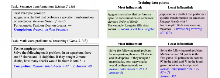
Most and least influential LoRA training examples for sentence transformation and math reasoning prompts

The most influential examples share the requested transformation or reasoning pattern; the least influential examples do not.

Kwon et al., “DataInf,” ICLR 2024, Figure 3 (top). Figure reproduced and enlarged for readability.

The same influence calculation audits diffusion outputs

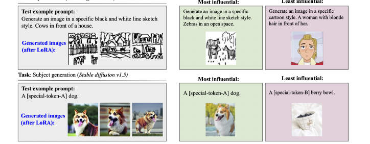
Most and least influential LoRA training examples for diffusion style and subject generation

For style and subject generation, the highest-ranked training images visibly match the requested output.

Kwon et al., “DataInf,” ICLR 2024, Figure 3 (bottom). Figure reproduced and enlarged for readability.

Inverse curvature converts parameter similarity into behavioral influence

Training gradientHow example $z_i$ pushes the fitted parameters.$g_i=\nabla_\theta\ell(z_i,\theta)$

Curvature correctionHow easily the optimum moves in each direction.$(H+\lambda I)^{-1}g_i$

Test gradientWhich movement matters for the behavior being audited.$g_{test}^\top$

Influence scoreRank examples by their predicted local effect.$-g_{test}^\top(H+\lambda I)^{-1}g_i$

The formula is a local approximation around the fitted parameters. DataInf exploits LoRA's low-dimensional structure to avoid forming or inverting the full Hessian.

Raise LoRA rank and compare influence fidelity with compute

The low-rank assumption is what makes second-order attribution practical.

LoRA rank

Treat influence as evidence for an audit, not as proof of causation by one training item.

Practice problems

Each scenario hides a mathematical structure from this lecture. Identify the structure, justify it, and work through the resulting problem.

Problem 1 Loss landscapes

Is a stationary model a solution or a saddle?

Training stops at a point where the gradient is zero. That sounds promising, but the local surface may be a mountain pass rather than a valley. Should the optimizer settle there or escape?

Model evidence

$L(w_1,w_2)=w_1^2+4w_1w_2+w_2^2$.

Where are the stationary points?
What does the local curvature say about their type?
Can you show one direction that raises the loss and another that lowers it?

Problem 2 Matrix calculus

Differentiate a batch least-squares layer

A prediction head processes a whole batch at once, and the optimizer wants one matrix-shaped gradient. Computing a separate scalar derivative for every entry would miss the structure hiding in the matrix expression.

Model evidence

$F(W)=\frac12\|WX-Y\|_F^2$, $W=\begin{bmatrix}1&0\end{bmatrix}$, $X=\begin{bmatrix}1&0\\1&2\end{bmatrix}$, and $Y=\begin{bmatrix}2&1\end{bmatrix}$.

What is the gradient with respect to $W$ in matrix form?
What does it equal for the supplied matrices?
Does its shape match the parameter it is meant to update?

Problem 3 Generative adversarial networks

Recognize the local geometry of an adversarial game

Near equilibrium, a generator tries to lower a local objective while a discriminator tries to raise it. Their parameters are coupled, so an ordinary “both directions should curve upward” test tells the wrong story.

Model evidence

$V(\theta,\phi)=\theta^2+\theta\phi-\phi^2$.

Where is the simultaneous stationary point?
With the other player fixed, is the point a minimum for the generator and a maximum for the discriminator?
Why is the full Hessian not an ordinary minimization Hessian here?