Concept Erasure and its Motivation
Concept erasure is a straightforward idea: we want to remove a specific concept from the learned representations of a model. In doing so, we must ensure that all other unrelated information in those representations remains untouched. But why would we need to erase something that has already been learned?
Consider a scenario where CVs are processed through a language model to generate embeddings for a downstream machine learning task. How can we guarantee the model relies solely on professional information rather than gender features encoded within those embeddings? Without specific constraints, we cannot be certain that the algorithm’s decision-making is free from unwanted information. A guaranteed solution is to remove gender-related information from the embeddings before performing the analysis.
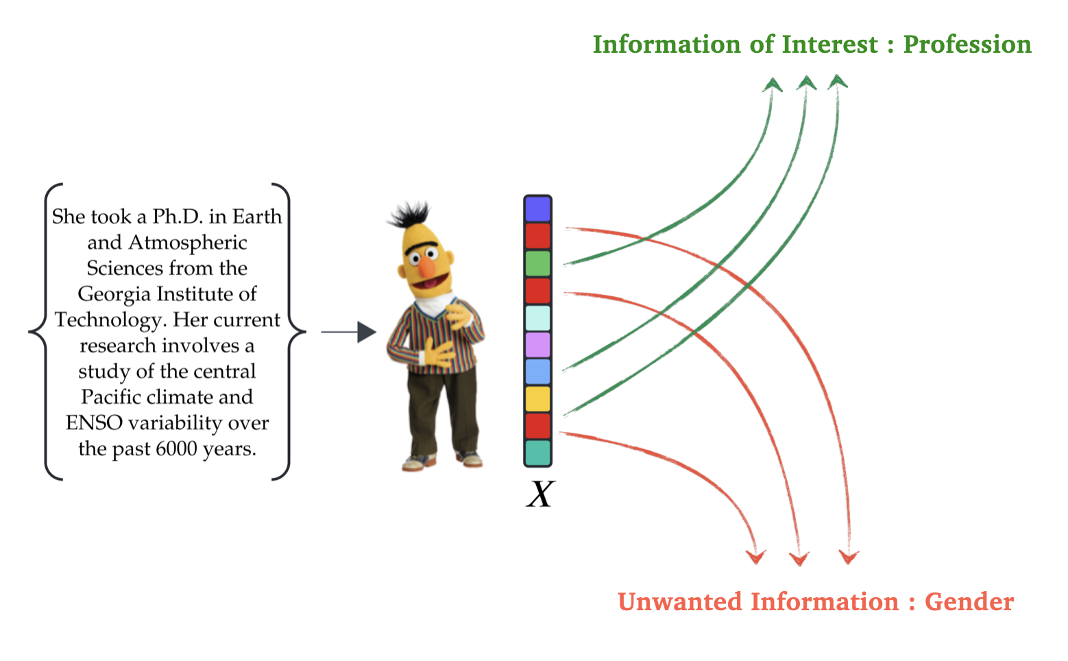
We should also note that during the training of large-scale models, we have minimal control over the specific information they encode. Furthermore, different downstream tasks may necessitate the removal of different types of information. Since retraining a foundation model for every unique requirement is impractical, it is more effective to develop methods for controlling the information within learned representations. Concept erasure studies this control, which can be applied either during training or afterward. The latter approach, known as post-hoc erasure, is our focus here.
Challenges in Concept Erasure
There are generally two challenges in concept erasure. First, we need a proxy to quantify how the unwanted concept and the learned representation are tied together. Second, we must delicately untie the unwanted information from the representation so that all unrelated information remains intact after erasure.
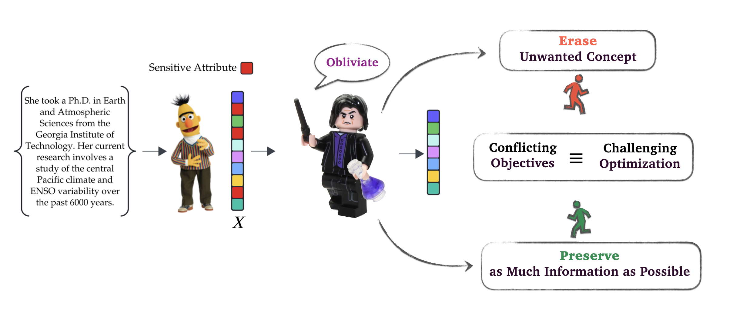
This makes the optimization problem for erasure quite difficult. On one hand, we want to remove information; on the other, we want to preserve information. Balancing these two competing objectives is challenging, and it is unlikely that, without a careful optimization setup, we will obtain a satisfactory result from this competition.
Utility-Erasure Trade-off
To evaluate the practical challenges of concept erasure, we examine the performance of current methods. Ideally, if a representation is free of a specific attribute (e.g., gender), it should be impossible to classify that attribute from the embeddings. Consequently, if a classifier maintains substantial accuracy post-erasure, the process is incomplete. This failure typically stems from optimization complexities or an inadequate proxy for measuring the dependency between the representation and the unwanted attribute.
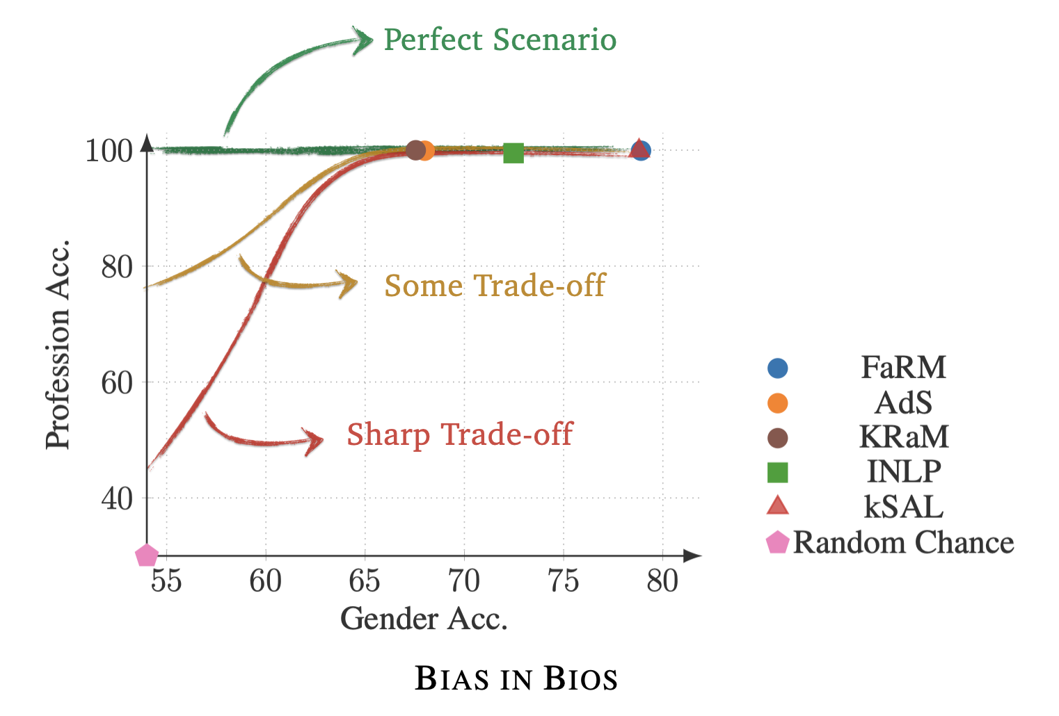
The figure illustrates gender erasure on the BiasInBios dataset. While methods like FaRM and KSAL leak significant gender information, KRaM and AdS are more effective. However, their 68% accuracy remains notably higher than the 53% random-chance baseline (majority class) for this dataset.
It is very likely to see a decline in utility accuracy as a concept is erased, as we expect a trade-off between utility and erasure. This trade-off profile reveals the dynamics of the competition between information removal and preservation throughout the erasure process. Analyzing this profile, rather than a single point as the final step of erasure, provides a more comprehensive evaluation of the underlying optimization approach used to formulate the erasure problem. Furthermore, when total erasure significantly degrades downstream performance, we can select a specific point along this trade-off curve that offers a better balance between utility and the leakage of unwanted attributes.
Nonlinear Guardedness
Now, let’s examine what complete erasure looks like in practice. The figure below illustrates Obliviator’s performance on the same dataset discussed earlier. These representations achieve approximately 62% accuracy for gender and 92% for profession.
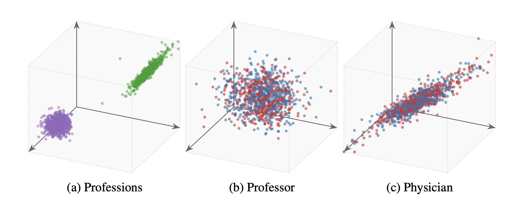
On the left, we see the distribution for professions, specifically physicians (green) and professors (violet). The adjacent plots show the gender distribution within each profession. As illustrated, the gender distributions within each class completely overlap, leaving no gender-related variation. Now, we can guarantee no downstream model can utilize gender-relevant information in its decision-making.
Erasure Means Statistical Independence
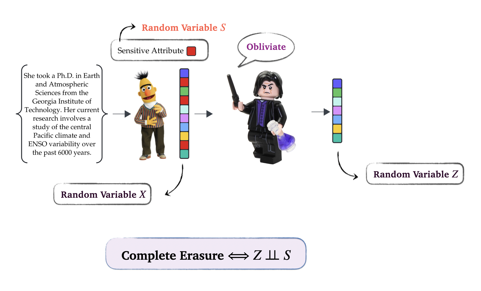
In the context of statistical learning, we treat embeddings and unwanted concepts as Random Variables (RVs), assuming access to samples from their joint distribution. This implies that for each embedding, the corresponding concept is known. Before erasure, a dependency, whether linear or non-linear, exists between these two variables. For erasure to be complete, this dependency must be eliminated. Mathematically, the erased representation must be statistically independent of the unwanted concept. Consequently, any method capable of quantifying and manipulating the statistical dependency between two RVs serves as a valid proxy for erasure, which can then be framed as the minimization of this quantity. However, the efficiency of the underlying optimization remains critical, as concept erasure is not just about removal but rather preserving essential information for the downstream task.
The Cost of Independence
Statistical dependency between two RVs, such as $X$ and $Y$, does not necessarily imply that we can directly predict $X$ from $Y$ or vice versa. For instance, if $X$ has a uniform distribution over $[0,1]$, but conditioning on $Y=0$ shifts $X$ to a Gaussian-like distribution with mean $0.5$ and variance $0.01$, then $X$ and $Y$ still exhibit statistical dependency. Fundamentally, two RVs $X$ and $Y$ are statistically independent if and only if $P(X|Y)=P(X)$. That is, knowing $Y$ does not alter the distribution of $X$, meaning the underlying random processes generating each RV are entirely decoupled.
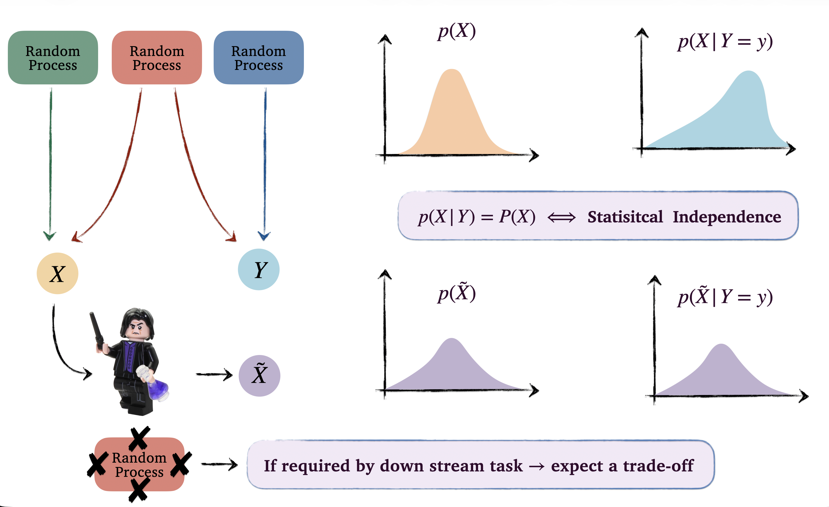
Now, consider the figure above, where two RVs $X$ and $Y$ share a random process, and we want the transformation $Z=f(X)$ to be independent of $Y$. Note that $f$ cannot change the fact that the origins of $X$ and $Y$ are entangled. Therefore, to achieve independence, $f$ must explicitly remove the effects caused by the shared random process in $X$ and $Y$. If the downstream task requires information from that shared process, this removal will inevitably degrade performance. This is the fundamental mechanism behind the utility-erasure trade-off.
A Functional Perspective on Statistical Dependence
Various mathematical frameworks exist to formulate statistical dependence. In information theory, for instance, mutual information is commonly used to quantify the dependence between two random variables (RVs). Alternatively, we can characterize this dependence through the lens of moments and functions.
Consider a random variable $X$ with bounded support (for example, $a \leq \lVert X \rVert \leq b$). If all moments of $X$ are unaffected by another RV $Y$, meaning $\mathrm{E}[X^k \mid Y] = \mathrm{E}[X^k]$ for every integer $k$, then we can conclude $P(X \mid Y) = P(X)$.
Usually, we reach for Pearson correlation or covariance. But covariance only captures first-order linear relationships. Even if we achieve mean independence, $\mathrm{E}[X \mid Y] = \mathrm{E}[X]$, this only guarantees $\operatorname{Cov}(X,Y) = 0$, not full independence in general.
To conclude true statistical independence, we can generalize from moments to function spaces:
\[X \perp\!\!\perp Y \iff \operatorname{Cov}(f(X), g(Y)) = 0, \quad \forall f,g\]Suppose $\mathcal{F}$ and $\mathcal{G}$ are function spaces rich enough to approximate continuous functions well. Then statistical independence can be written as:
\[\sup_{f \in \mathcal{F}} \sup_{g \in \mathcal{G}} \left|\operatorname{Cov}(f(X), g(Y))\right| = 0\]By selecting these spaces as characteristic RKHSs, we can express covariance through a cross-covariance operator:
\[\operatorname{Cov}(f(X), g(Y)) = \langle g, \operatorname{Cov}_{YX} f \rangle_{\mathcal{G}}\]This leads to Hilbert-Schmidt Independence Criterion (HSIC):
\[\operatorname{HSIC}(\mathcal{F}, \mathcal{G}, P(X,Y)) = \left\|\operatorname{Cov}_{YX}\right\|_{HS}^{2}\]and, with characteristic kernels,
\[\operatorname{HSIC}(\mathcal{F}, \mathcal{G}, P(X,Y)) = 0 \iff X \perp\!\!\perp Y\]Functional Approach In Action
Consider two RVs
\[X = \sin(Z) + \epsilon_x, \quad Y = \cos(Z) + \epsilon_y,\]where $Z \sim U(-\pi,\pi)$ and $\epsilon_x, \epsilon_y \sim \mathcal{N}(0,1)$ are independent noises. Here, $X$ and $Y$ are dependent through shared $Z$, even though linear covariance can be close to zero.
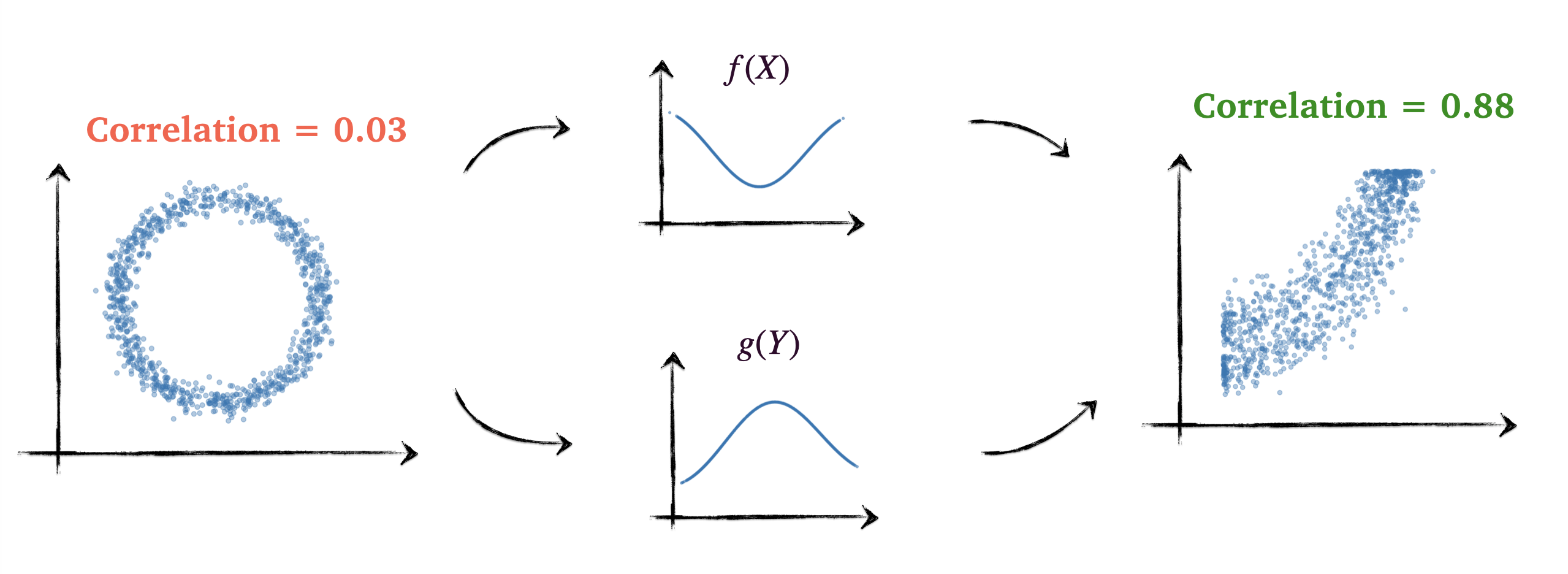
We can search for functions $f$ and $g$ that reveal this hidden dependency by maximizing covariance:
\[\sup_{f \in \mathcal{F}} \sup_{g \in \mathcal{G}} \operatorname{Cov}(f(X), g(Y)) \quad \text{s.t.} \quad \|f\|_{\mathcal{F}} = \|g\|_{\mathcal{G}} = 1\]The norm constraints keep the problem bounded. Intuitively, this optimization finds transformations that make the dependency between $X$ and $Y$ as linearly visible as possible.
Why Functional Approach ?
Thus far, our discussion assumes access to the underlying distribution. In practice, we usually only have finite samples: embeddings, sensitive labels, and possibly utility labels.
The functional approach avoids explicit density estimation and instead relies on expectations that can be estimated empirically. In finite samples, we approximate an infinite-dimensional cross-covariance operator with a finite-rank matrix, and accuracy improves with more data.
A key factor is smoothness of the chosen functions $f$ and $g$. In RKHS, smoothness is controlled by norm constraints and kernel choice. Poor kernels can overestimate or underestimate true dependency.
Erasure via Functional Approach
Because HSIC captures broad dependency patterns, we can formalize erasure. Let $S$ be the unwanted concept, $Y$ the downstream utility, and define erased representation
\[Z_\theta = \epsilon(X;\theta),\]where $\epsilon$ is a guarding function.
We optimize:
\[\inf_{\theta} \Big(\operatorname{HSIC}(Z_\theta, S) - \operatorname{HSIC}(Z_\theta, Y) - \operatorname{HSIC}(Z_\theta, X)\Big)\]“Maximizing dependency” here does not create new information. It makes already-shared structure more detectable so the optimization preserves useful information while removing unwanted dependency.
Suboptimality of Vanilla Optimization Setup
While the objective above is principled, a single-stage optimization is often unstable. In practice, it can oscillate, be sensitive to initialization, and converge to inconsistent points on the utility-erasure curve.
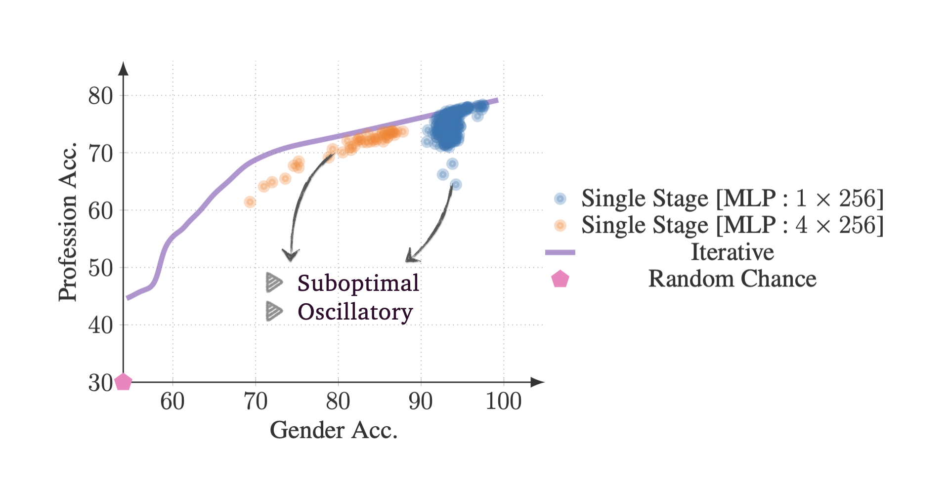
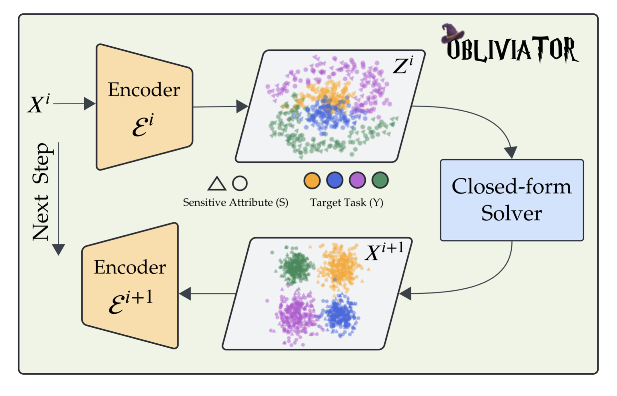
The iterative trajectory in the figure corresponds to the behavior of Obliviator.
Motivations Behind Obliviator
Obliviator solves erasure iteratively, gradually transforming representation space and smoothing competition between objectives.
As erasure progresses, clusters associated with the unwanted concept move toward overlap. In high-dimensional spaces there are many ways this collapse can occur, but only some preserve unrelated utility structure. Standard gradient descent on the single-stage objective is unlikely to find the least-destructive path by itself.
Why do preservation terms not guarantee full preservation? Because HSIC is a sum over squared singular values of a cross-covariance operator. Optimization tends to preserve dominant modes first, potentially sacrificing weaker but still useful structures.
Intervening in the Erasure Optimization
A useful strategy is to intervene when unrelated structures start collapsing. The idea is to realign representation space so utility-relevant structure stays more visible than unwanted concept structure.
Following the functional view, define a visibility metric for the unwanted concept:
\[\sup_{g} \operatorname{Cov}(f(X), g(S))\]In constrained optimization, we aim to keep this quantity at zero. This does not imply full statistical independence, since invertibility of $f$ is not guaranteed. Full independence would require:
\[\sup_{g} \sup_{h} \operatorname{Cov}(h(f(X)), g(S)) = 0\]That nested form is intractable in practice, so the first metric is used as a practical constraint.
Obliviator: Smooth Concept Erasure
Now we define an intervention objective for finding $f$ during optimization. Suppose $Z^i$ is the representation at current iteration, $X$ comes from the previous iteration, and $X_i$ is the current input. Similar to the earlier functional setup:
\[\sup_{\{g_I\}} \sup_{f} \Big( \operatorname{Cov}(g_{x_i}(X_i), f(Z_i))^2 + \tau_x\operatorname{Cov}(g_x(X), f(Z_i))^2 + \tau_y\operatorname{Cov}(g_y(Y), f(Z_i))^2 \Big)\]subject to
\[\sup_{g_s}\operatorname{Cov}(g_s(S), f(Z_i)) = 0, \quad \|g_I\|_{\mathcal{G}_I} = \|f\|_{\mathcal{F}} = \|g_s\|_{\mathcal{G}_s} = 1.\]This yields an eigenvalue problem, letting us explicitly keep dependency modes above a tolerance $\epsilon$.
By introducing intermediate RVs and multiple preservation terms, optimization is less likely to collapse onto only the easiest dominant mode. The augmented encoder objective becomes:
\[\inf_{\theta} \Big(\operatorname{HSIC}(Z_\theta, S) - \operatorname{HSIC}(Z_\theta^{i}, Y) - \operatorname{HSIC}(Z_\theta^{i}, X) - \operatorname{HSIC}(Z_\theta^{i}, X_i)\Big)\]In summary, Obliviator decomposes single-stage erasure into a multi-stage iterative loop: an encoder optimization step followed by an eigenvalue-based intervention step that realigns representation space.